Numerical simulations are commonly if not routinely required for composite insulators equipped with grading/corona rings to ascertain electric fields in three sensitive areas: on the grading/corona ring and end fittings; on the housing surface; and at the triple point where air and housing meet the metallic end fitting. The main purpose is to assess risk of deep erosion related to water droplet corona. This degradation is considered critical since erosion on a composite insulator sheath can progress down to the fiberglass core and result in brittle fracture or other failure modes.

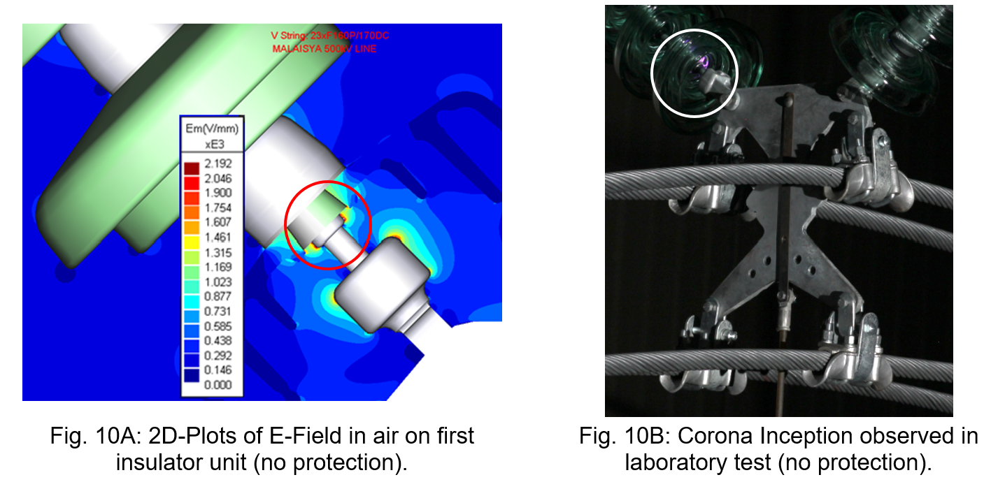
The situation is much different, however, for toughened glass (or porcelain) cap and pin insulators, whether with or without an RTV coating. Here, the above approach is usually not considered by end users since absence of a fiberglass core avoids such a concern. Rather, the only characteristic to consider is the visible corona inception voltage, which is directly related to the electric field in the air surrounding an insulator string and to the voltage grading along this string.

Sediver has had long experience in E-Field calculations going back to the late 1980s and now uses Finite Element Analysis (FEA) of electric field distribution and voltage grading to validate and secure design of insulator strings as well as complete assemblies with hardware and fittings. This work currently uses COMSOL.

This edited contribution to INMR by Frédéric Delhumeau, Technical Assistance Engineer, Cédric Dumas, CAD Technician and Jean Marie George, Scientific Director at Sediver review interesting examples of such work on insulator strings for AC overhead lines.

---

1. FEA Methodology

It is worth as a start to present the overall process of a Finite Element Analysis (FEA), which can be synthesized as follows:

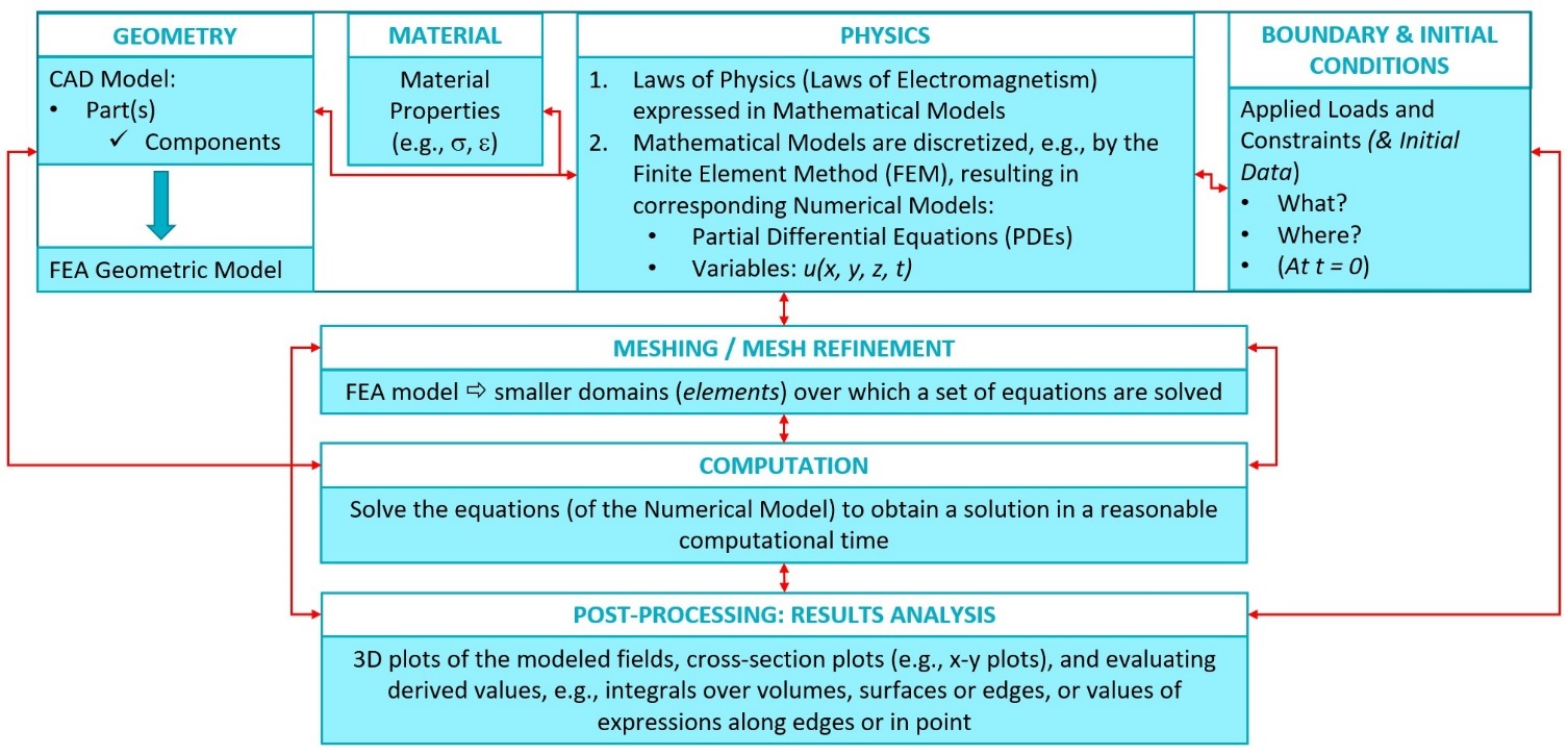
FEA is usually an iterative process: it starts with a simple model that includes the geometry, the material(s), the physics and the boundary conditions. This model can be fine-tuned step-by-step, thereby increasing its complexity and/or level of detail. Each iteration is worked out keeping a balance between two opposing criteria: On the one hand, the model shall be fine or detailed enough so that the computed solution will approach as much as possible the “true solution”; on the other hand, the model shall be coarse or light enough so that the numerical model is able to converge in a reasonable computational time without any error when solving the equations. Red arrows in the flowchart represent possible forward/backward flows between different steps of the process.

The appropriate “physics” shall be defined first. Most software solutions available exhibit a large library of physics models. Among those covered by the fundamentals of Electromagnetics and described by Maxwell’s equations, the following physics may be considered and evaluated:

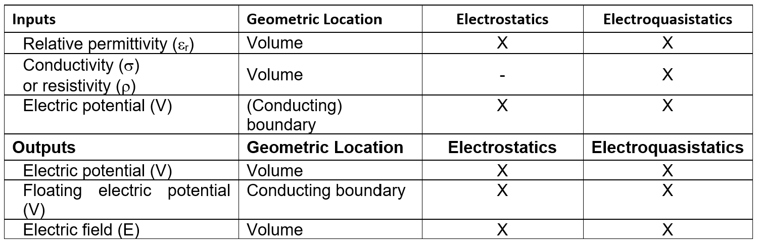
Electrostatics: This is the sub-field of electromagnetics describing an electric field due to static (non-moving) charges. As an approximation of Maxwell’s equations, electrostatics can only be used to describe insulating, or dielectric, materials entirely characterized by electric permittivity. When performing an electrostatics analysis, any conducting materials (typically metals) are first removed from the analysis and the metallic surfaces are seen as exterior boundaries from the perspective of the dielectric materials.

Steady Currents: This analysis is used to compute the steady current flow in highly conductive materials such as metals. An electronic current is driven through a conductor by a difference in electric potential. The material in a steady currents analysis is completely characterized by its electrical conductivity. When performing a steady currents analysis, any insulating materials are first removed from the analysis and the insulating surfaces are seen as exterior boundaries from the perspective of the conductive materials.

Electroquasistatics: This analysis is a generalization of electrostatics and steady currents in cases where magnetic effects can be neglected. It is only possible to combine the capacitive effects of electrostatics with the conductive effects of a steady currents analysis if the fields are time varying. If there is any time variation in e.g. voltages at the boundaries, total current is the sum of a conduction current and a displacement current. Conduction current density is associated with electric conductivity and displacement current density is associated with electric permittivity. Electroquasistatics can be seen as a dynamic version of the steady current equations with an additional contribution from the displacement current.

Two of these three analyses are of particular interest and Table 1 presents typical inputs and outputs for those.

Various numerical methods have been developed to obtain solutions for electromagnetic field problems. There are two different kinds of solution methods, i.e. using either differential equations or integral equations. The former is known as the ‘domain method’ and the second is known as the ‘boundary method’.

Domain methods are based on differential equations and on discretization of the whole domain by regular grids or elements. The finite difference method (FDM) and the finite element method (FEM) are the most familiar domain methods. Research discussed here has been based on the FEM.

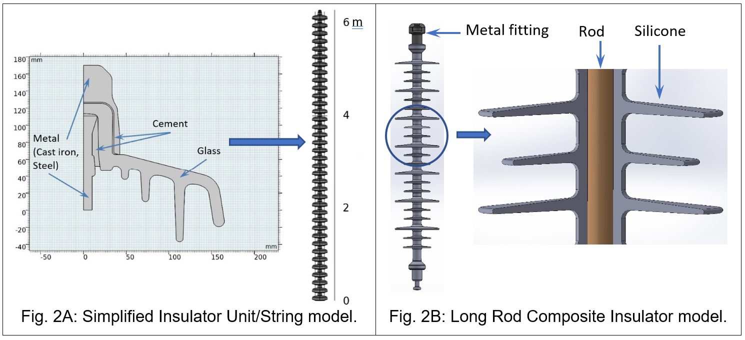
The complexity of the geometry of a complete insulator strings assembly (set) with fittings shall be thoroughly assessed before performing a FEA.

First, and in contrast to a long rod composite (or porcelain) insulator, an insulator string (without hardware) combines multiple parts of different materials. These have various and complex shapes with dimensions in the range of a few millimeters or centimeters and resulting in a complete “heterogeneous structure” with dimensions up to more than several meters.

Some simplification of this geometric model may become necessary depending on the objective of the FEA. With regard to assessment of Electric Field distribution and voltage grading along insulator strings:

• the detailed designs of the ball and socket coupling and of the split pin locking device of the insulator units can be simplified as long as this ensures a continuous voltage distribution;
• all the hardware and fittings constituting the complete assembly can be modeled by simplified but representative metallic parts. However, when used, arcing protection devices such as arcing horns, rings, rackets shall be modeled accurately since they have significant impact on electric field distribution and voltage grading;
• all the parts that constitute the geometric model, primarily the insulator units, hardware and fittings, may exhibit “singularities”, such as screws, nuts, split pins, sharp angles, sharp edges, recesses, etc. that may result locally in numerical results that do not account for “real-world behavior”. These “singularities” can be simplified and not considered in the FEA. The FEA will not accurately compute electric field that could be induced locally around or near these “singularities”, but which might induce corona/RIV activity during laboratory testing or in service, if inappropriately designed or manufactured.

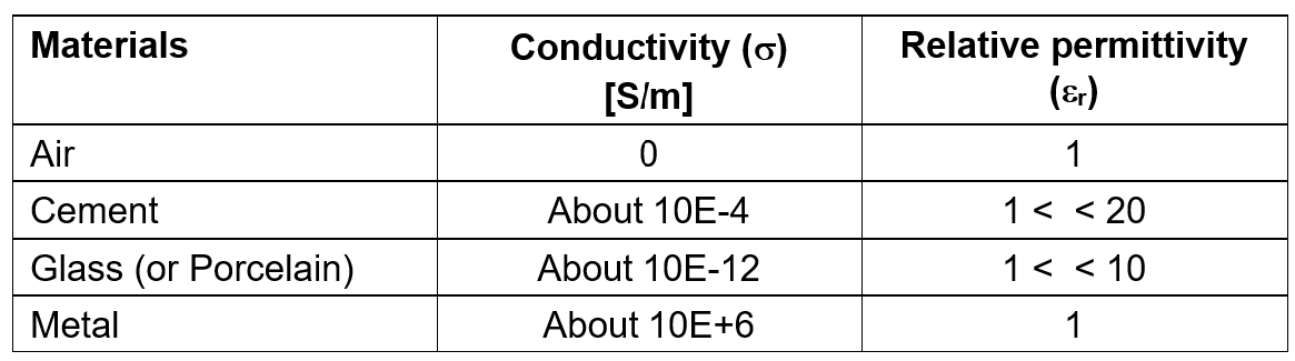
Moreover, a complete insulator set with fittings can combine multiple materials with different characteristics; Typical magnitudes of such properties are illustrated in Table 2. Properties of insulating parts, i.e., toughened glass (or porcelain) associated with the cement shall be thoroughly documented or characterized.

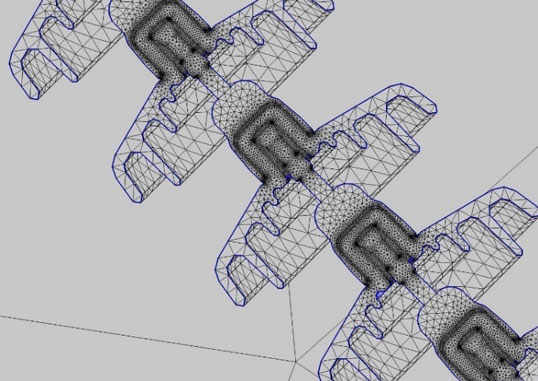
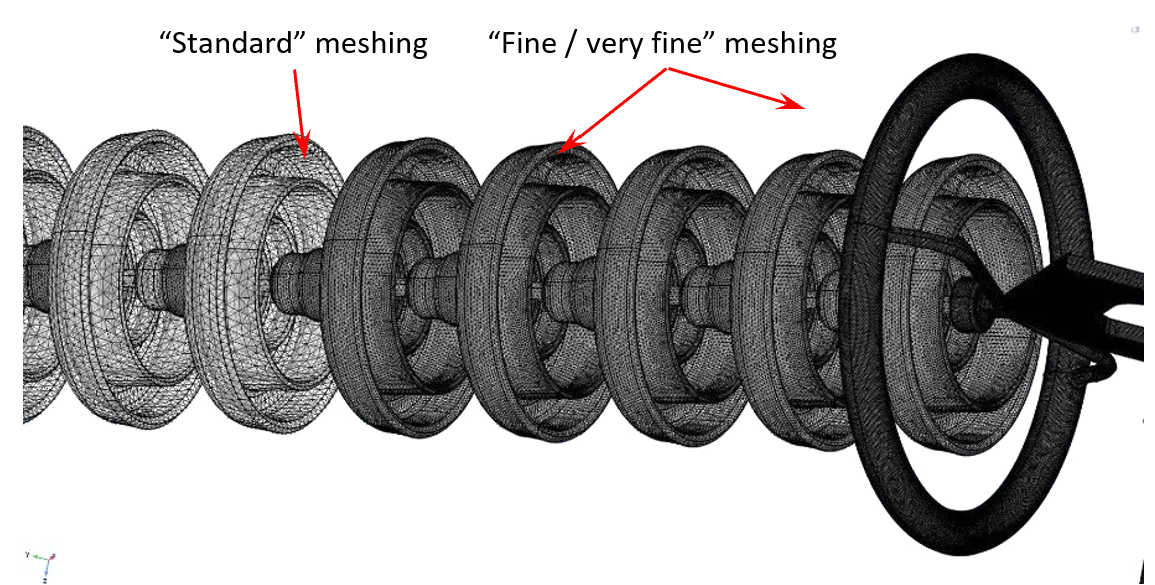
The geometric model can be meshed automatically by the software, as shown in Fig. 3. The accuracy of the results that can be obtained from any FEA model is strongly related to the finite element mesh used. The “physics-controlled” meshing is an option to take into consideration not only the geometry and the materials of the different parts and their components but also the “physics” to solve.

Various techniques such as global or local adaptive mesh refinement can be applied to improve accuracy. Fineness of the mesh is directly and primarily dependent on the scale and degree of accuracy of the geometric model.

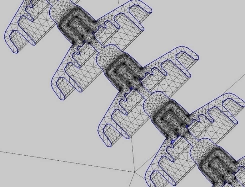
For FEA on complete insulator set with fittings, meshing can be refined in all the parts close to energized conductors, in particular insulator units and arcing protection devices close to the energized conductors, as shown in Fig. 4. The purpose is to achieve more accurate results in the areas where highest electric field can be expected and where possible corona inception is more likely to occur.

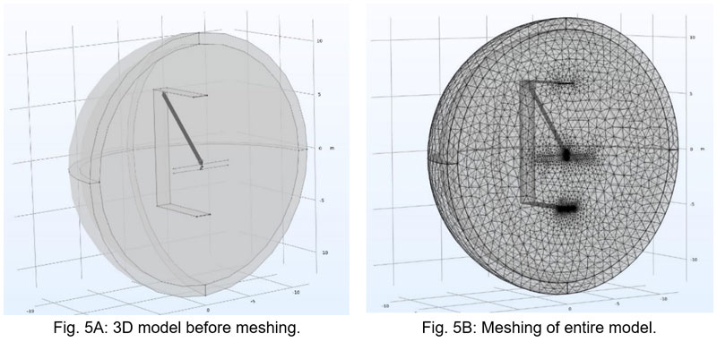
For illustrative purposes, Fig. 5A and B show an example of the complete model of a V-suspension set in the central window of a suspension tower before and after meshing. Since it is an insulating material (gas), a sphere of air and of “infinite” diameter (or volume) was modeled all around the insulator assembly, conductor bundles and tower model. To simplify the numerical computation by reducing computation time and risk of numerical errors, geometric symmetry planes of the actual assembly were considered.

2. FEA Process Validation: Comparison with Laboratory Testing

To evaluate representativeness and accuracy, an FEA was worked out on a simple insulator hardware assembly and the results compared to those obtained by laboratory testing.

The insulator set considered consisted of a single I-suspension string of 10 units connected with simple fittings to a conductor (modeled by a tube) of given length and hung to a cross-arm. Figs. 6A to 6C show the 3D-geometric model used in the FEA as well as the test set up. The FEA was carried out using the latest version of COMSOL Multiphysics software, in particular the AC/DC module specialized in low-frequency electromagnetics modeling and computation. The computation was based on the Electric Currents formulation with Conservation of Currents in the (low) frequency domain (50-60 Hz).

A key question arises: What relevant parameter(s) need to be considered to compare numerical simulation to laboratory measurement?

• Electric field: It is the primary cause of possible corona inception, which is associated with appearance of conductivity of a gas (i.e. air) in the environment of an insulator set (or conductor) brought to high voltage. It is well-known that intense electric fields that may occur at the surfaces of “live” components of the insulator set can under some circumstances lead to ionization and electrical breakdown of the air immediately surrounding these parts. However, the laws of physics, and the mathematical and numerical models of available software solutions do not address or account for this phenomenon of air ionization and appearance of such corona.
  Moreover, accurate measurement in the laboratory (or on an operating overhead line) of electric field distribution around an insulator string is not (or is only hardly) accessible. Measurement of corona inception in a laboratory is based on examination. Even if techniques such as light amplification or a corona camera can be used to allow more accurate measurement, examination of corona inception on “actual” parts depends greatly on factors such as local shape and dimensions, surface quality, etc. that are not easily addressed by the numerical simulation implemented.
• Voltage grading (in kV or % of applied voltage) along each insulator of the string. Although not covered by any international test standard, this distribution can be measured in the laboratory using a sphere-gap device and also obtained from a numerical simulation.

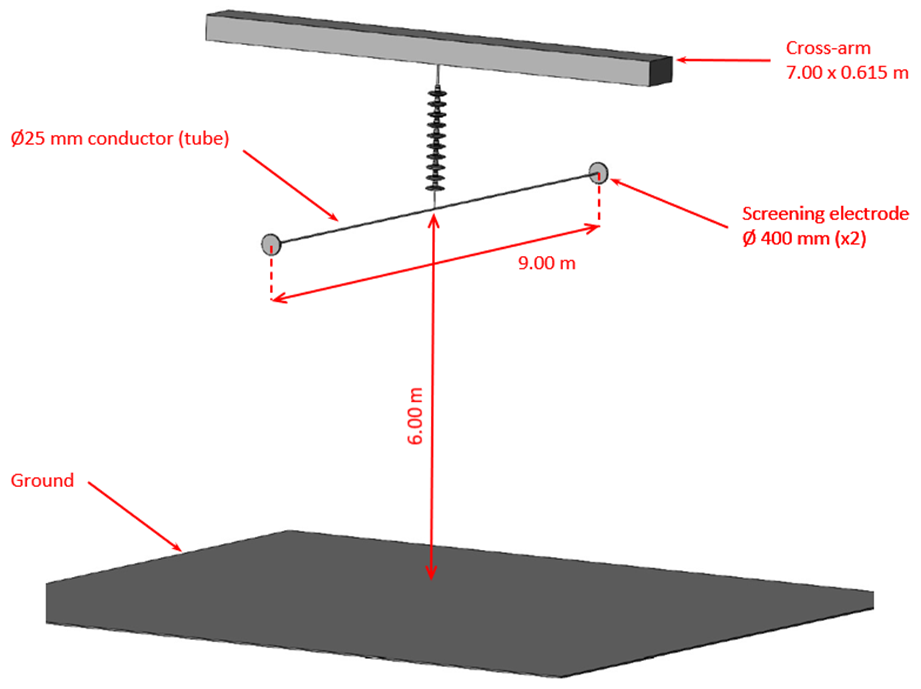
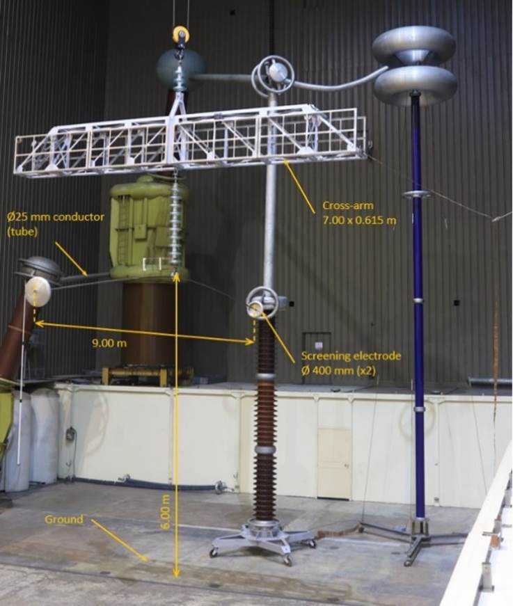
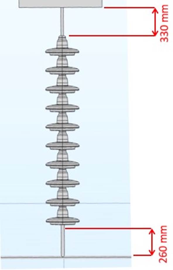
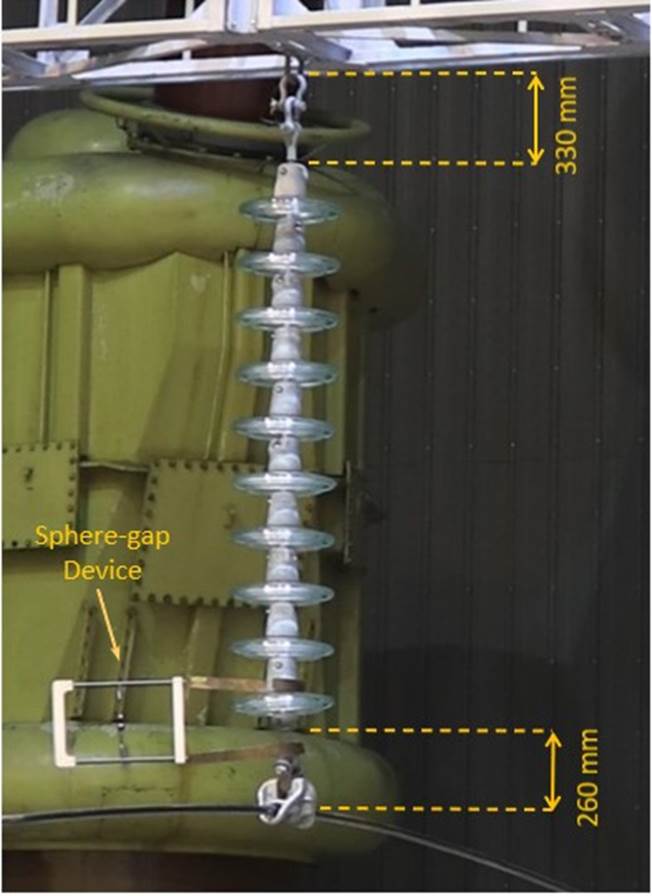
Fig. 6F compares the voltage distribution (in % of applied voltage) across each insulator unit obtained from numerical computation (in blue) and also by laboratory measurement (in green).

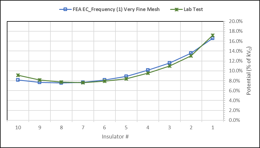
Considering the uncertainty inherent in any test method, this study showed good consistency and a small difference (i.e. less than one percent) between numerical and experimental result, which is negligible.

3. What to Expect

Use of FEA can be of great benefit to validate and secure the design of insulator sets for an overhead transmission line. Some examples based on real case studies are presented below:

3.1 Example 1: Effect of Protections
A first example analyses the effect of arcing protection devices at the live end of a V-suspension set. For any given number of insulator units per string and conductor arrangement, comparative simulations were worked out respectively without and with protection rackets or rings.

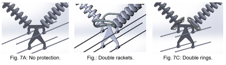
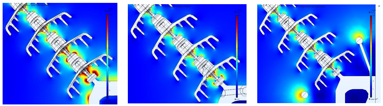
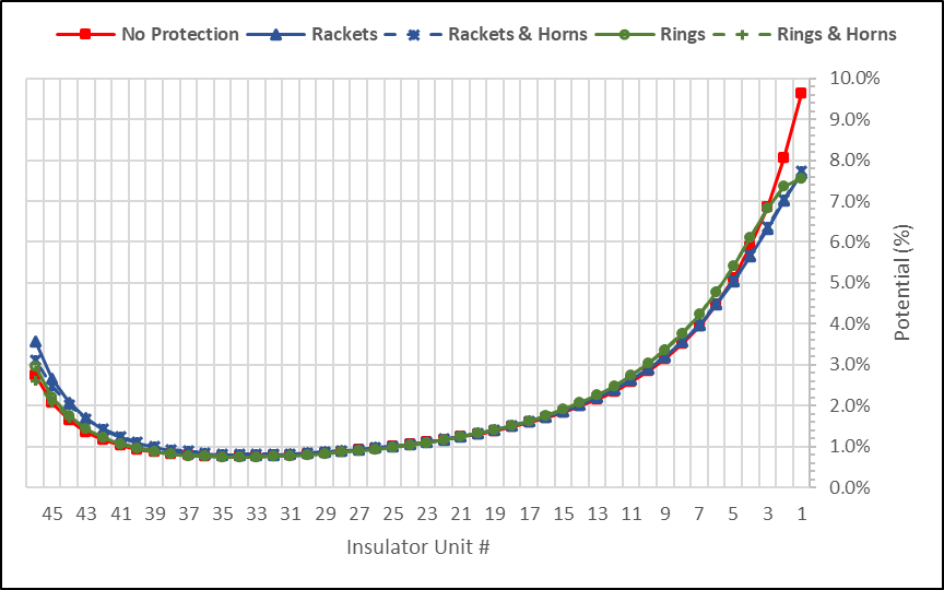
Computations clearly show the effect of protections in reducing both E-Field and voltage grading at the bottom sides of the strings. In this particular example, for example, arcing rings were found slightly more effective than rackets. Additional laboratory tests revealed good consistency between areas of highest calculated electric field and examination of corona inception location.

3.2 Example 2: Effect of Number of Insulators per String
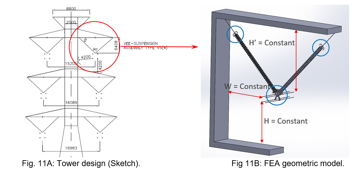
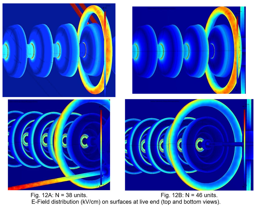
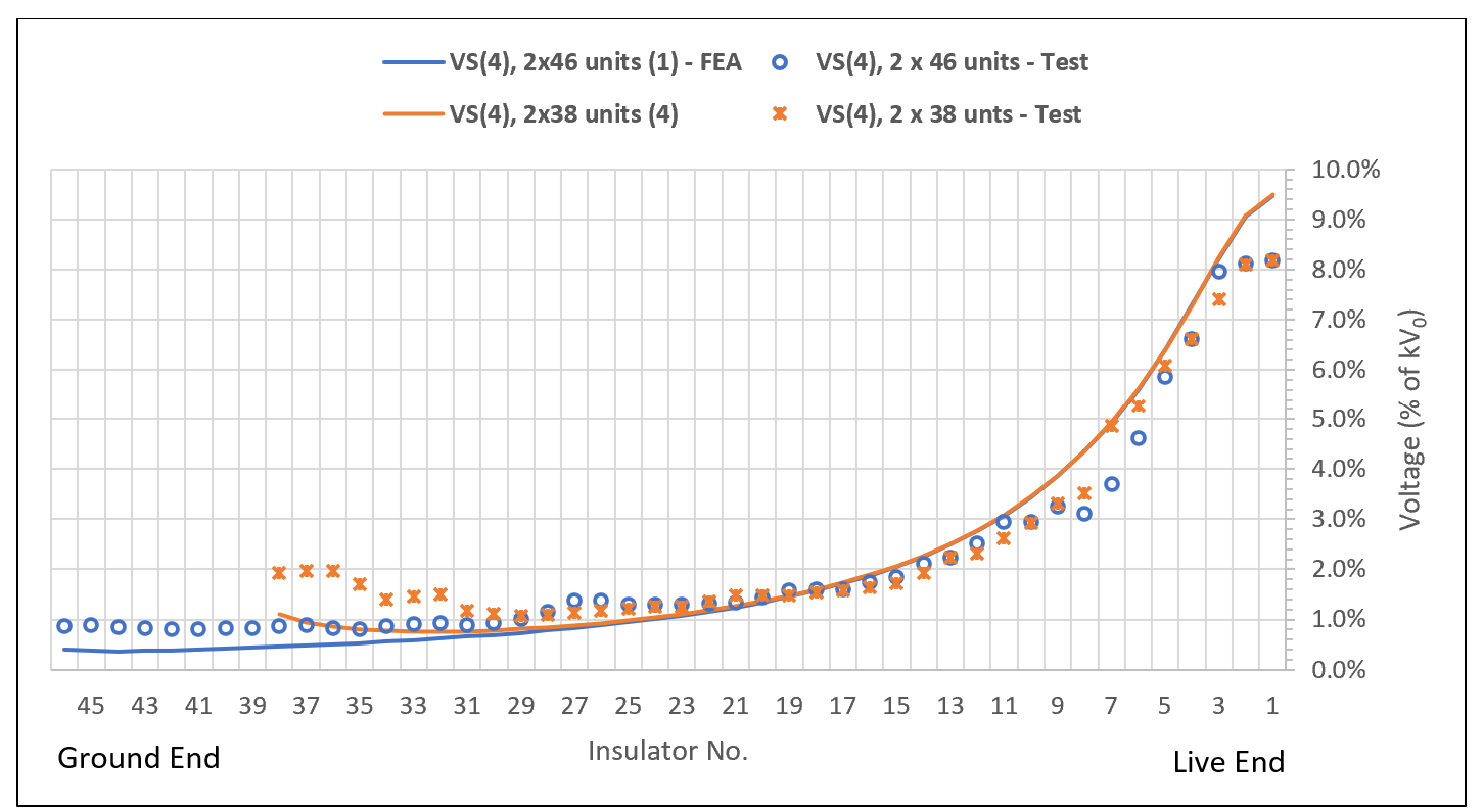
A second example illustrates the effect of number of insulator units in a V-suspension string in the lateral phase of a suspension tower. In this example, the V-suspension set is equipped with arcing horns at the ground end and arcing rings at the live end. The length of the extension links connecting the first insulator unit (at ground side) to the tower cross-arm is adjusted according to number of insulator units in the string such that the overall dimensions (i.e. width and height) of the insulator set are constant and the distances of the conductor bundle to the tower (i.e. cross-arms and vertical plane) are also constant.

From this FEA, no significant difference in E-Field distribution and voltage grading was observed at the live end of the set (close to the conductor bundle). On the opposite end, although the values were relatively low, the increase in number of insulator units allowed reducing electric stresses. This result was confirmed by a voltage distribution test in the laboratory.

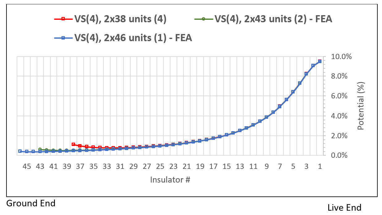
Reasonably good consistency in voltage grading was further observed between numerical simulation and laboratory testing.

3.3 Example 4: Effect of Conductor Bundle Arrangement
This example studied influence of design of the conductor bundle arrangement on E-Field distribution at the bottom of the insulator strings. For a given V-suspension set, a triple and a quad arrangement of conductor bundle of the same spacing were analyzed and compared.

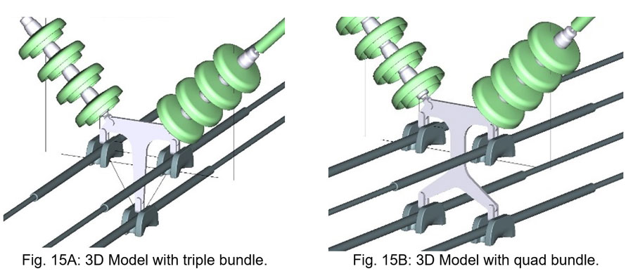
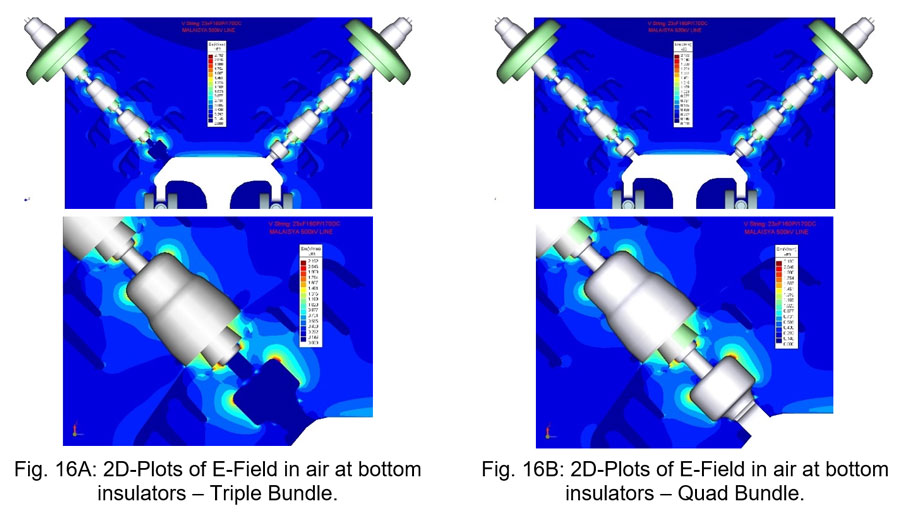
In this example, no significant differences were found in E-Field distribution at the bottom of the strings. E-Field is affected primarily by the upper two sub-conductors of the bundle rather than by the lower one(s).

3.4 Example 5: Effect of Tower Grounding (Suspension Sets)
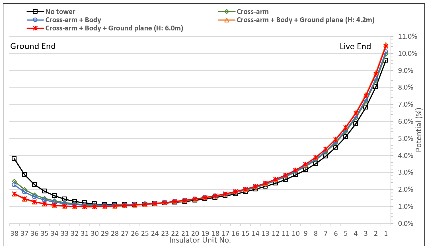
This example studied the “grounding” effect of the tower on voltage distribution (and E-Field distribution) along a suspension insulator string. The aim was to define the appropriate “size” and complexity of the geometric model that is suitable for a representative and accurate FEA. Considering a V-suspension set design with a constant number of units, the following simulations were performed:
1. V-suspension set without attachment fittings (such as extension links) and without tower. See Fig. 17A.
2. V-suspension set with extension links connecting the upper ends of the insulator strings to a horizontal cross-arm. See Fig. 17B.
3. The same model as above but adding a vertical plane simulating the tower body. See Fig. 17C.
4. The same model as above but adding a horizontal plane underneath the conductor bundle, simulating the grounded cross-arm of the lower phase. See Figure 17D. Two distances (H1 and H2) were consdiered between the two lower sub-conductors of the bundle and the bottom grounded cross-arm.

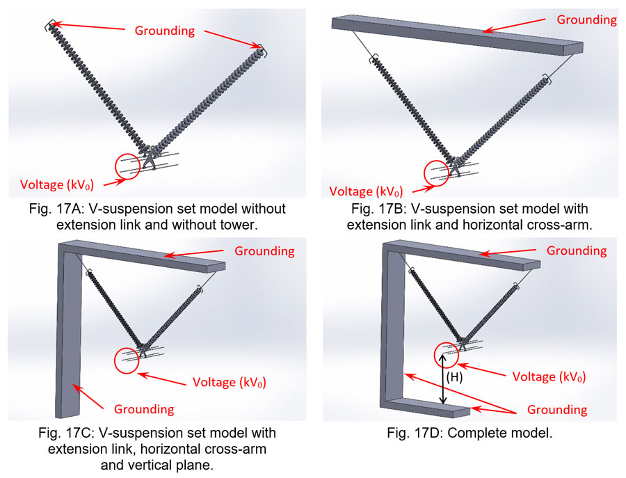
The voltage grading curves below clearly show that the tower lowers the voltage primarily at the ground end of the strings, i.e. along the 8 to 9 last (upper) units: The curve (in black) without any tower modeling exhibits the highest voltage, whereas the curves with complete tower modeling exhibit the lowest voltage. On the other end, voltage grading increases slightly at the live end when tower modeling is added.

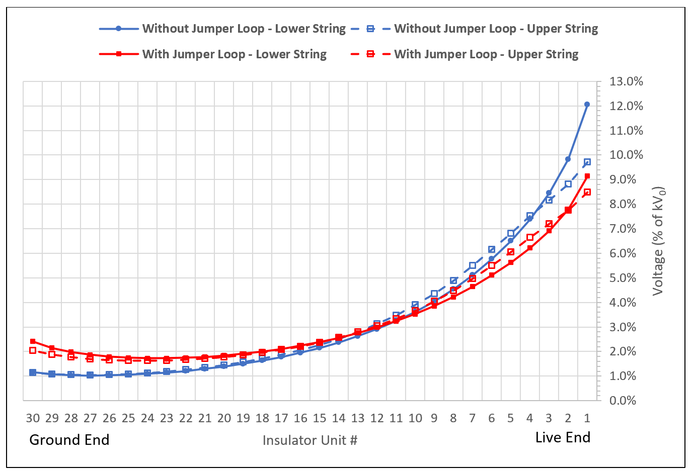
3.5 Example 6: Effect of Jumper Loops (Tension Sets)
As under real conditions where these are oriented towards the forward or back conductor spans on either side of the tower, simulations for tension insulator sets can be performed with only a horizontal plane representing the tower cross-arm to which they are attached. However, the effect of the jumper loops connecting the sets on either side must not be overlooked.

In this study, a triple tension set with one arcing ring at the live end was modeled, with and without jumper loop.

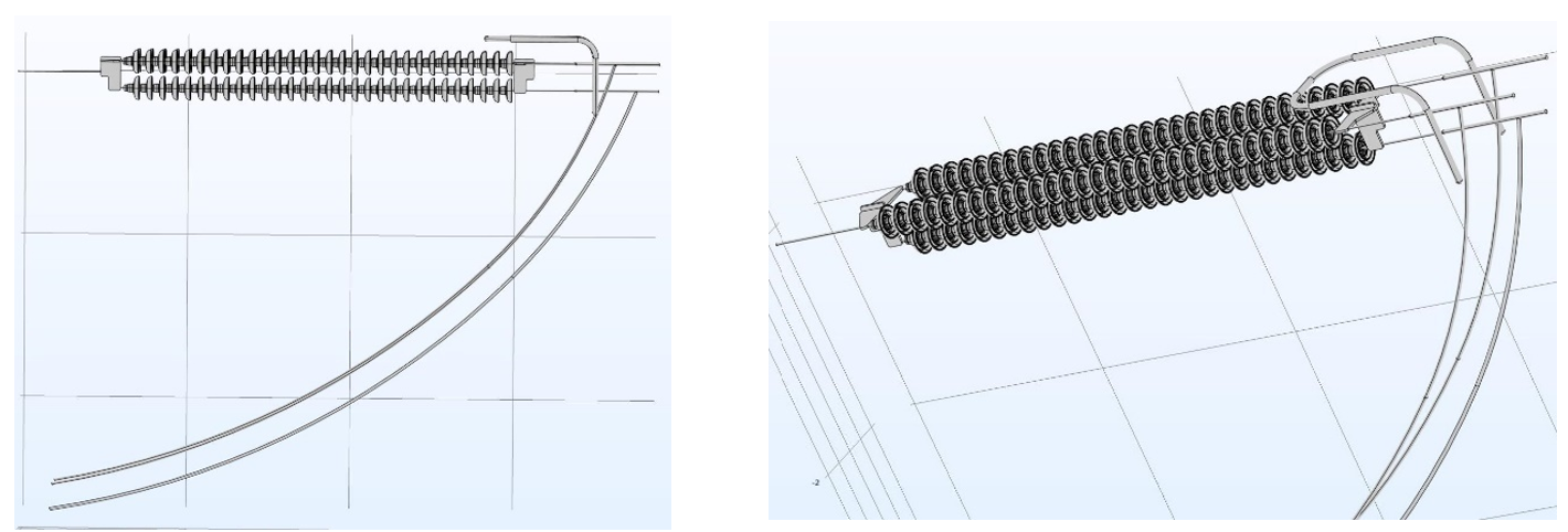
The computation showed that the increase in voltage across the insulator units at the live end decreased as the energized conductors of the jumper loop get closer to the strings. The beneficial effect of arcing rings above the upper insulator strings compared to the lower string was again also confirmed.

4. What Not to Expect: FEA Limitations

These simulations were worked out on insulator units in a dry and clean condition. As such, pollution phenomena were not considered. Nor was an RTV silicone coating on the toughened glass (or porcelain) shell surface considered since this does not significantly impact E-field but rather primarily leakage current should pollution be present.

Moreover, all these numerical simulations of electric field and voltage grading were based on Maxwell’s Equations of Electromagnetism. Those do not take pollution phenomena into consideration, primarily dry band arcing under pollution.

At present, with today’s knowledge in this field, no physical or mathematical models and no standard procedure have yet been established to simulate a polluted surface where the contaminant deposited can be more or less uniform in thickness, more or less evenly distributed over the surface, more or less conductive, more or less dry, unevenly wet, etc. Moreover, the dynamic nature of dry band arcing can simply not be considered in any static or quasi-static simulation.

[inline_ad_block]