This edited past contribution to INMR by Dr. William Chisholm explained how transmission line surge arresters provide a supplement to traditional lightning protection using overhead groundwires and the natural impedance of tower footings in soil. TLSAs represent a cost-effective alternative to installation of supplementary buried ground electrodes in some cases where improved performance is required. They also provide a means to retro-fit lightning protection to lines that, for various reasons, were constructed without sufficiently effective countermeasures. However, a successful application of TLSA to improve power quality must fit into the context of overall line reliability, considering geographic features including local soil resistivity and exposure to lighting as well as other causes of flashovers in a multi-factor insulation coordination process.
Utilities are called to respond to findings such as:
• Some two‐thirds of the overall annual cost of poor power quality to the U.S. economy has related to momentary interruptions of electric power systems;
• Nearly 60% of the annual cost of power quality problems to the European Union economy has related to voltage dips and short transients;
• Individual EU countries have reported minimum annual cost of voltage dips in the range 4.5 to 17 € per inhabitant; and
• Customer investment of €700k to deal internally with voltage dips between 65% and 90% of nominal, with duration less than 150 ms, have a payback period of 3 months, while investment of €2500k to deal with dips to less than 65% of nominal voltage have had a payback period of 5 to 12 years.

Voltage Dip and SARFI Definitions
Generally, at the customer level, a voltage dropout or interruption to a small fraction of line voltage that lasts a short time, for example less than 20 ms, is acceptable. After this time, a much smaller dip, for example to 70% of nominal, is tolerated. The “retained voltage” throughout a dip event is the smallest one-cycle rms voltage, recomputed on a half-cycle basis for ac systems. The “duration” is the time difference from the beginning to end of voltage sag, which starts when the voltage drops below 90% of nominal and ends when it recovers above 91%.
There are common definitions of voltage sag and duration in IEC 61000-4-30, IEC 61000-2-8 and IEEE P1564. Some utilities make use of time-sag plots, tabulating surge duration in intervals. For IEC and UNIPEDE, the time intervals are defined as follows: (<0.1 s, 0.1-0.25 s, 0.25-0.5 s, 0.5-1 s, 1-3 s, 3-20 s, 20- 60 s, 1-5 min). Voltage intervals are taken in 10% increments of nominal from 0 to 90%. In South Africa, the NRS-0480-2 standard simplifies the sag duration/magnitude classification based on duration of (20 to 150 ms, 150 to 600 ms, 600 ms to 3 s) as well as magnitude (0 to 40%, 40-60%,60-70%, 70- 80%,80-85%,85-90%). Other utilities simplify further by counting the voltage dip/duration events that fit above or below the traditional ITIC/CBEMA or SEMI-47 curves to obtain a System Average RMS Variation Frequency Index (SARFI – ITIC) or (SARFI –SEMI).
Cost of Avoided Voltage Disturbances
One motivation for quantifying the number of disturbances from lightning outages on transmission systems is that overhead groundwire (OHGW) protection sets out a utility-specific benchmark for the financial value of avoiding a customer voltage disturbance. The utility has invested, on behalf of all its consumers, a sum on the order of 5 to 10% extra to provide the OHGW conductors and also to support them with taller towers, suitably strengthened to resist the additional overturning moment forces. For each line, overall number of flashes can be readily estimated using standard methods such as CIGRE Brochure 63 or the IEEE Standard 1243TM FLASH program. Using the normal assumption that every shielding failure on a transmission system will result in a flashover and phase-to-ground fault, the incidence of disturbances without OHGW can be simply computed from the flash incidence using the height of the uppermost phase conductor. No correction is needed for first-stroke currents that are too weak to cause a flashover in this calculation. A weak first stroke in a flash is likely to be succeeded by one or more subsequent strokes of sufficient magnitude to cause flashover, even for EHV insulation levels. This means that the flash rate to the line gives a close estimate of the number of transmission line flashovers that would have occurred if the line had no OHGW.
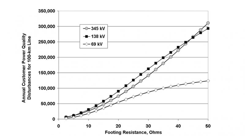
Using a series of simplifying assumptions about constant customer and transmission line loads, as well as the North American model that every phase-to-ground fault on the transmission line leads to a voltage dip of more than 20 ms duration and falling below 70% of nominal voltage, Fig. 1 suggests that the annual number of customer dips increases nearly linearly with the average footing resistance of a transmission line.
The simple customer Power Quality (PQ) disturbance estimate in Fig. 1 suggests that the voltage level of the transmission line can change from 138 kV to 345 kV without much change in effect. While outage rates on 345 kV systems are lower, because the OHGW protection is more effective, the number of customers affected by the outage scales with both the system voltage (2.5 times higher) and the line current in bundle conductor (3 times higher) compared to 138 kV lines with single conductors.
The utility cost to avoid a large fraction of the potential momentary customer PQ disturbances, through the use of OHGW protection, ranges from $US 0.01 to $1 per customer dip, depending on voltage level, phase arrangement and local ground flash density. Some baseline measures of the customer costs of preventable voltage dips from 1995 suggested that the $US 1 level, or $US 0.4 per kW of load, was appropriate for residential customers but that for commercial and industrial loads, a higher cost of $3-$4/ kW was associated with momentary outages. By 2001, for example, the high average cost of a fault-and- successful-reclose sequence, related to damage to customer equipment as well as resetting of digital systems, emerged as an important power quality issue in the USA, independent of energy delivery considerations.
In some countries, the first phase-to-ground fault from lightning does not lead to a severe customer disturbance. At present, the number of customers affected by a voltage dip on a transmission system, and their actual costs from the disturbance, remain open questions. These questions are being resolved with suitable accuracy on a country by country basis, using results from power quality monitors, coordinated with transmission system operator records of faults and supplemented with measurements of radiated fields from lightning location systems.
Relation Between Lightning & Voltage Dips
The “reach” of a voltage dip in response to a transmission line flashover and its successful clearing by automatic reclosing, is an interesting ac power quality issue. In cases where the fault is in a series path between generation and load, lightning flashovers and reclosing times to clear the faults, generate voltage dips of sufficient depth and duration to be registered as problems in most power quality ranking schemes. However, when there are two or more transmission paths in a grid system, the power system response is established by re-computing currents and voltages. In either case, of radial feed or meshed grid, lightning remains a major root cause of flashovers, especially on transmission systems up to 250 kV.
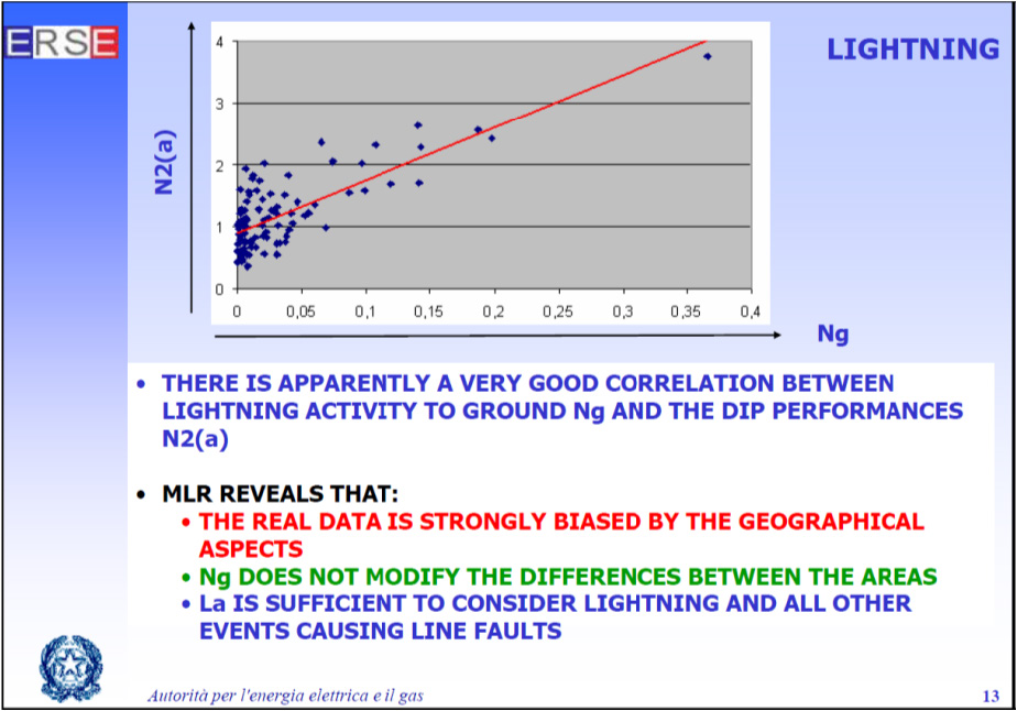
Recent work in voltage dip monitoring in Italy evaluated details of the relationship between a disturbance measure, N2(a), and lightning ground flash density, Ng, with findings shown in Fig. 2.
Flash density is approximately constant over the length of a typical transmission line and considering line length La alone as a root cause may be sufficient. In fact, Fig. 3 supports this as it shows that the average annual total (cloud + ground) flash density is constant through most of Italy. Based on optical transient density (OTD) measurements, the total flash level is 6 < OTD < 8 flashes/km2/year, and is observed to rise above 10 flashes/km2/year only in the north.
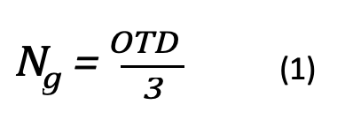
Estimated ground flash density Ng = OTD/3.
The recommended expression to convert OTD to ground flash density, correcting for the fractions of cloud and ground flashes as well as their relative optical intensities, is:
 This conversion suggests a ground flash density of 2 < Ng < 2.7 flashes/km2/year in most regions, and rising to Ng > 3.3 only in the north of Italy. Estimates of ground flash density based on thunder, also shown in Fig. 3, should no longer be used as the uniform coverage of satellite observations gives a much more detailed and statistically valid estimate in areas where lightning location network observations are not available.
In addition to regional and annual variations in Ng, there are strong regional variations in soil resistivity in many countries. For example, in Italy, where there is a wide regional variation of power quality [20] in spite of relatively constant flash density, Fig. 4 shows that there is also a wide variation in ground conductivity. Measurements in Fig. 4 are based on 1-MHz signal attenuation and suggest soil of high 30 mS/m conductivity (33 Ωm resistivity) in the northeast, along with areas of 0.3 mS/m (3300 Ωm) and more extensive regions of 1 mS/m (1000 Ωm) in the mountainous north and southwest.
Areas of low conductivity are more vulnerable to distribution system flashovers from nearby lightning. This will have a direct effect on the number of power quality issues related to the path from distribution station to customer. For larger‐scale transmission paths, these regional changes in ground conductivity translate into corresponding variations in the median footing resistance of typical lines in different areas. For the same size of tower foundation, doubling the conductivity will reduce the footing resistance by half, and Fig. 4 thus suggests that there can be 30:1 differences in resistance depending on region in Italy. In regions of 0.3 mS/m conductivity, it is technically difficult to obtain satisfactory 20 Ω footing impedance in soil with for typical transmission tower foundations, even with supplemental buried ground electrodes nearby.
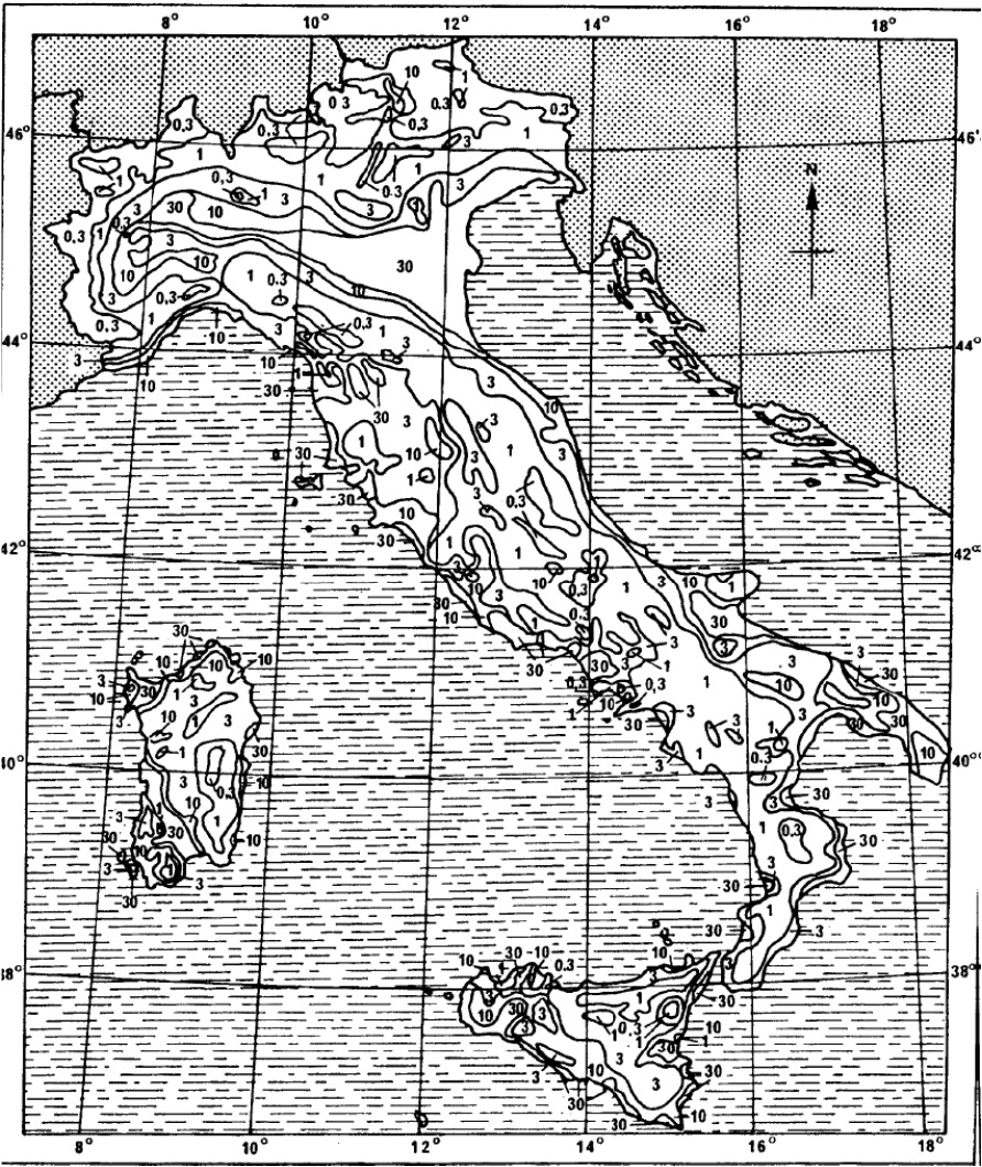
Soil conductivity κ (mS/m) in Fig. 4 is related to soil resistivity ρ (Ωm) by the relation = ρ1000/ κ.
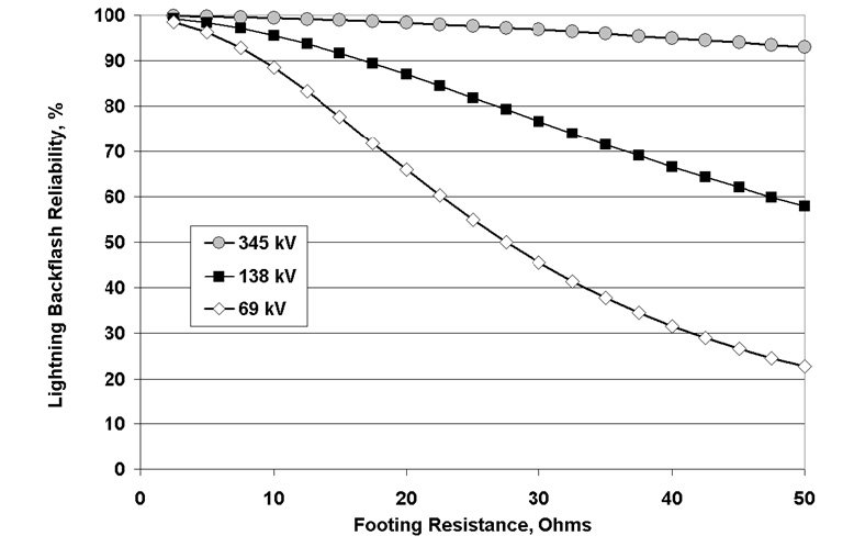
As shown in Fig. 5, a doubling of the footing resistance from 20 to 40 Ω on average is predicted to decrease the effectiveness of a double overhead groundwire (OHGW) protection system from 87% to 66% for a 138-kV line. The lightning tripout rate, and the number of faults per unit of ground flash density, would increase by a factor of (1-0.66)/(1-0.87) = 2.6 times with 40 Ω resistance compared to 20Ω. This dependence of transmission system outage rate on footing resistance, which is in turn a linear function of soil resistivity, illustrates why lightning flash density alone, in Fig. 3, cannot fully explain some regional variations in power quality.
Tower-to-Tower Variation of Footing Resistance
In addition to changes in soil conductivity with region, there are large tower‐to‐tower variations in the soil. This affects the size of foundation and sometimes the type of tower, and also plays a role in the optimization of arrester use.
Some regions have thin soil cover over underlying rock, with a highly variable depth of overburden that provides most of the effective resistivity. In one airborne resistivity survey, the standard deviation of the logarithm of resistivity σln ρ at 100 kHz, measured at each tower, was found to be about 0.6 for short line sections and 1.2 < σln ρ < 1.4 for longer sections of 68 to 83 towers. This compares with a value of σln I = 0.48 used to summarize all observations of negative peak first return stroke current I in lightning flashes.
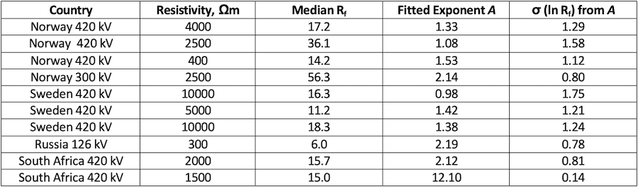
The wide variability of soil resistivity can also be inferred by studying the statistics of tower footing resistance measurements. In cases where the utility does not modify the towers at construction to improve values observed above a preset limit, footing resistance also seems to be log‐normally distributed. In Tennessee, USA, the standard deviation of ln(Rf) was in the range of 0.90 to 1.46, with a median of 0.92. Similar distributions of footing resistance in South Africa, Norway and Sweden also suggest a natural value of σln Rf > 1.0 in Table 1.
The practice of extending the grounding systems at towers whose natural footing resistance does not meet a pre‐defined threshold, such as 20 or 25 Ω, can change the shape of the distribution, leaving the values below the threshold unchanged and reducing those above the threshold by a factor of two.
Simplified Statistical Insulation Coordination Processes
The empirical fits in Table 1 take advantage of a simple approximation to the log-normal distribution, used widely for the parameters of lightning strokes:
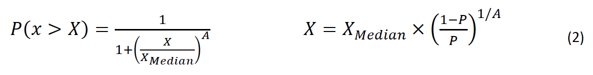
This is an easily inverted and acceptable approximation, when limited to the probability range of 1% < P< 99%. When restricted to this range, there is a unique and useful relation between the exponent A in Equation 2 and the standard deviation of the natural logarithm σln X: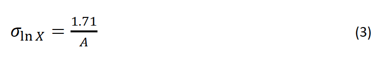
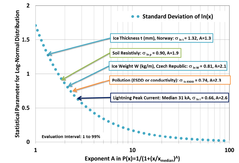
The use of A=2.6 in Equation (3) along with a median first return stroke peak current of 31 kA in North American lightning practice corresponds to σln I = 0.66, which is close recommended value in for the backflash regime in which Ipk > 20 kA. This point, along with values of A fitted to observed distributions of soil resistivity and other insulation coordination parameters, is illustrated in Fig. 6.

The insulation coordination problem for lighting involves multiplying scaled distributions of two parameters, peak current and soil resistivity. Each parameter has a rather wide range of variation that can be described by a log-normal distribution or approximated using Equation 2, twice, once for the impressed current and a second time to obtain the local tower resistance. Every insulator on a stricken tower is subjected to a different lightning impulse voltage stress, depending on the position of the supported phase relative to the OHGW as well as the instantaneous line voltage. Usually, one insulator will have the highest impulse voltage from tower to phase. The insulation strength will follow a volt- time curve with a time related to span length. The resulting flashover voltage has a linear normal distribution with low 3-5% standard deviation.
Some other insulation coordination problems involve a single environmental parameter with a wide statistical variation. For example, the line voltage is constant, and the relative standard deviation of flashover at a given level of contamination for constant line voltage is on the order of 4 to 8%. This means that Equation 2 only appears once, to describe the log-normal probability that equivalent salt deposit density (ESDD) exceeds a threat level. However, there is a complication that the number of insulators exposed to contamination may be higher – on the order of 3 to 300 for a line section and as many as 1000 insulators in parallel at large substations.
The threat level for ESDD is fixed by the line voltage stress, divided by the leakage distance to obtain E50 in kV rms of line to ground voltage per meter of leakage distance. The critical flashover level is then given for example by:
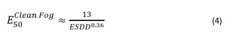
where ESDD is in units of mg/cm2.
The corresponding process for insulation coordination across iced insulators, like lightning protection, calls for multiplying together two separate distributions: one of ice thickness, and another of the electrical conductivity of the precipitation. The resulting icing stress product (ISP), expressed in μS/cm × g/cm, is related to the critical flashover gradient E Heavy Ice by:
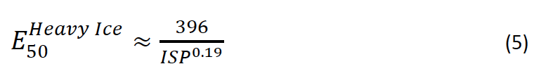 where E Heavy Ice is in units of kV rms of line to ground voltage per meter of leakage distance.
This simplified process has not been applied or evaluate to describe all risks of insulator flashover. In cases of bird streamer pollution, the conductivity is fixed but the streamer volume and length vary depending on the size of the bird. Water flux from ocean spray or drift overspray from cooling towers is a function of distance, wind speed and direction, which have natural random variations. In these two cases, however, the applied water conductivity is fixed at 4 mS/m or 4000 μS/cm respectively.

Optimizing Insulation Coordination with Arresters
Grounding improvements will give a well‐defined reduction in customer momentary disturbances, as illustrated in Fig. 1. A utility facing power quality challenges can use the benchmark life‐cycle cost of these improvements, considering installation, inspection and replacement, to evaluate the optimum use of line surge arresters as an alternative.
There are several strategies to applying the line arresters.
The first, and easiest to explain to stakeholders, is to simply fit arresters across every insulator, with the expectation that lightning outage rates will drop to zero. The capital investment of this alternative may be funded by a stakeholder other than the utility, directly or under the terms of a performance improvement contract. This can be an optimal political choice, rather than the best technical solution.
A second strategy is to apply the arresters selectively, to all insulators of one or more phases uniformly along the line. For example, fitting arresters to the bottom two phases of a vertical double circuit line can eliminate backflashovers at these highly stressed positions, located far from the OHGW. This treatment also reduces stress on nearby phases and improves the overall performance of the line by raising the “threat current” that just causes flashover at each tower, whatever its local value of footing resistance.
For transmission lines in areas of low conductivity (≤ 0.3 mS/m), there will be individual towers and line sections where it is difficult to achieve a footing resistance that is low enough to allow the OHGW to function correctly. The required footing resistance varies with line voltage as shown in Fig. 5, from a “difficult to achieve” 5‐Ω requirement for 69 kV systems, up to 40 Ω for 95% effectiveness at 345 kV. In these regions, the optimal application of arresters will supplement OHGW protection at tower towers where the local soil resistivity is higher than average. Since the cost of grounding improvement is more‐or‐less fixed per tower, and the cost of a TLSA increases as a nonlinear function of the system voltage, this strategy is more effective at lower voltage levels. One factor in tower‐ by‐tower improvements is the need to bracket treated towers with arresters at adjacent towers that have sufficiently low resistance, in order to minimize transfer of flashover to unprotected phases nearby.
Arresters have been used to correct deficiencies in original tower head layouts with regard to shielding failures, for example in cases where a line was designed for two OHGW but only one side were strung, or has reached end of service life. For this duty, the arrester will carry a much larger fraction of surge current and will require a suitable energy rating and cross‐section. The extreme case of this application is the lower‐voltage line that was never fitted with OHGW, but must now meet regulated limits on the Momentary Average Interruption Frequency Index (MAIFI) or the SARFI defined previously.

Conclusions
Analysis of the optimal use of transmission line arresters to improve power quality should make use of both the ground flash density and the variation of soil conductivity within a region. In the insulation coordination calculations, it should be considered that the tower‐to‐tower variation of soil conductivity, resistivity and footing resistance have log‐normal distributions, with values of standard deviation that are as large as those associated with natural risks such as insulator contamination level, ice thickness or precipitation conductivity. Simplified methods can be suitable for approximating the log‐ normal distributions provided in a limited probability range of 1 to 99%.
References
[1] Hamachi-LaCommare, K. and Eto, J., “Cost of Power Interruptions to Electricity Consumers in the United States (U.S.)”, Lawrence Berkeley National Laboratory report LBNL-58164, February 2006, http://eetd.lbl.gov/ea/EMS/EMS_pubs.html
[2] Manson, J. and Targosz, R., “European Power Quality Survey Report”, Leonardo Energy Report, November 2008.
[3] Brekke, K., “4th Benchmarking Report on Quality of Electricity Supply – Voltage Quality Monitoring – Costs due to Voltage Disturbances”, Proceedings of CEER/EURELECTRIC Workshop on Voltage Quality Monitoring, Brussels, 18 November 2009.
[4] Walldén, B-A., “Problems and Measures with Voltage Disturbances at Skoghamm Mill”, Proceedings of CEER/EURELECTRIC Workshop on Voltage Quality Monitoring, Brussels, 18 November 2009.
[5] Bollen, M., “Joint Working Group C4.110 Voltage Dip Immunity of Equipment in Installations”, Proceedings of CEER/EURELECTRIC Workshop on Voltage Quality Monitoring, Brussels, 18 November 2009.
[6] Iglesias, J.L.G., “JWG CIGRE-CIRED C4.107, Economic Framework for Voltage Quality”, Proceedings of CEER/EURELECTRIC Workshop on Voltage Quality Monitoring, Brussels, 18 November 2009.
[7] IEEE, Guide for Improving the Lightning Performance of Electric Power Overhead Distribution Lines (Piscataway, NJ: IEEE), Standard 1410TM-2010, January 2011.
[8] IEC Standard 61000-2-8, Voltage dips and short interruptions on public supply systems with statistical measurement results, November 2002.
[9] IEC Standard 61000-4-11, Edition 2, Voltage dips, short interruptions and voltage variations immunity tests, March 2004.
[10] IEC Standard 61000-4-30, Edition 2, Testing and measurement techniques –Power quality measurement methods, October 2008. [11] IEEE Standard 1159TM -2001, IEEE Recommended Practice for Monitoring Electric Power Quality
[12] IEEE Standard 1366TM-2003, IEEE Guide for Electric Power Distribution Reliability Indices
[13] IEEE Standard Project P1564, Voltage Sag Indices
[14] CIGRE WG 01 of SC 33, Guide to Procedures for Estimating the Lightning Performance of Transmission Lines (Paris: CIGRE), Technical Brochure 63, Oct 1991.
[15] IEEE, Guide for Improving the Lightning Performance of Transmission Lines (Piscataway, NJ: IEEE), Standard 1243TM‐1997.
[16] Chisholm, W.A. and Anderson, J.G., Guide for Transmission Line Grounding: A Roadmap for Design, Testing, and Remediation, EPRI, Palo Alto, CA: 2004. 1002021.
[17] EPRI AC Transmission Line Reference Book, 200 kV and Above, EPRI, Palo Alto, CA: 2005. 1011974.
[18] Sullivan, M. and Keane, D., Outage Cost Estimation Guidebook, EPRI, Palo Alto, CA: 1995. TR-106082.
[19] Primen, The Cost of Power Disturbances to Industrial & Digital Economy Companies, EPRI, Palo Alto, CA: 2001. 1006274.
[20] Villa, F. and de Nigris, M., “Experience with VQM in Italy”, Proceedings of CEER/EURELECTRIC Workshop on Voltage Quality Monitoring, Brussels, 18 November 2009.
[21] NASA LIS/OTD Science Team, LIS/OTD 0.5 Degree High Resolution Full Climatology (HRFC), NASA/MSFC/GHRC, Huntsville, AL, USA, Version 2.2, http://thunder.nsstc.nasa.gov/data/, 1 September 2006.
[22] CCIR Recommendation 832, “World Atlas of Ground Conductivities”, 1982.
[23] Chisholm, W.A. and Williamson, J., “Issues in Long‐Term Reliability of Transmission Line Surge Arresters (TLSA)”, Proceedings of CIGRE Colloquium on Application of Line Surge Arresters in Power Distribution and Transmission Systems, Cavtat, May 2008.
[24] Chisholm, W.A., Petrache, E. and Bologna, F., “Grounding of Overhead Transmission Lines for Improved Lightning Protection”, Proceedings of IEEE Transmission and Distribution Conference and Exposition, New Orleans, LA, USA, 19-22 April 2010.
[25] Gutman, I., Haslan, K., Wallin, L., Solomonik, E., Vosloo, W.L. and Lundquist, J., “Line performance estimator software: Calculations of lightning, pollution and ice failure rates compared with service records”, Proceedings of CIGRE 2006, paper B2-205.
[26] Farzaneh, M. and Chisholm, W.A., Insulators for Icing and Polluted Environments (New York: Wiley, IEEE Press Series on Power Engineering), 680 pp., 2009.
[27] IEEE, IEEE Guide for Test Methods and Procedures to Evaluate the Electrical Performance of Insulators in Freezing Conditions (Piscataway, NY: IEEE), IEEE Standard 1783TM-2009, 17 October 2009.
[28] CIGRE Working Group C4.301, “Use of Surge Arresters for Lightning Protection of Transmission Lines”, (Paris: CIGRE), Technical Brochure 440, December