This second part of an edited contribution to INMR by Riccardo Bonanno and Michele de Nigris of RSE in Italy reviews research carried out to elucidate the phenomena behind recurring cable joint failures under climatic and electrical stresses. This work also assessed vulnerability of a medium voltage cable network and its components to weather extremes and aimed to identify measures to increase resilience of power systems under these circumstances.
A case study was conducted, involving a 185 mm2 Al, three-core XLPE cable. Cable temperature was computed based on the model developed and correlation was sought with the daily faults. The value of I represents the ampacity for the cable under consideration and the values shown in Table 1 are kept constant for the entire period of the simulation.
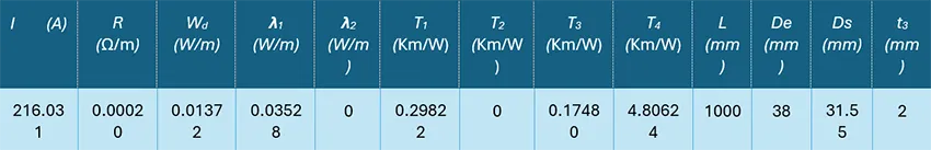
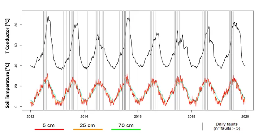
Application of the cable temperature model described by CEI EN 60287-1-1: 2001 is presented in Fig. 1. Temperature of the conductor during summer reaches values close or above 80°C during the hottest years. The trend of the conductor temperature reflects the trend of soil moisture in the third layer at about 70 cm, which is the one closest to the depth where the cables are usually placed.
This behavior is related to dependence of some terms of the equation on the soil thermal conductivity which in turn depends on moisture. It can also be seen that periods with the highest fault frequency do not coincide with the periods with highest conductor temperature but often with periods where conductor temperature has the steepest increase at the beginning of the summer, exceeding the threshold of about 50°C. Looking at Fig. 1, it is also clear that the most important factor determining faults seems to be the steepness of the conductor’s temperature curve. This is clearly noticeable considering the summers of 2012 and especially 2015.
Setting Up of Fault Prediction Model / Step 2: Implementation & Validation
Based on the correlations observed above, an overall fault prediction model was developed using Machine Learning (ML) techniques. These are considered most suitable to process non-linear relationships between predictive variables (providing that a sufficiently long time series of historical data of electrical faults associated with a specific threat to be studied is available).
Among ML methods, the Random Forest Method was used, which consists of generating an arbitrary number of simple decision trees, averaged to determine the result. The fault rate prediction model for underground cables over the city of Milan has been calibrated using an ensemble of variables (meteorological variables, load and temperature of a typical conductor discussed in Part 1 of this article), such as maximum load, soil skin temperature, ground temperature at the cable depth with its 10-day moving average, etc.
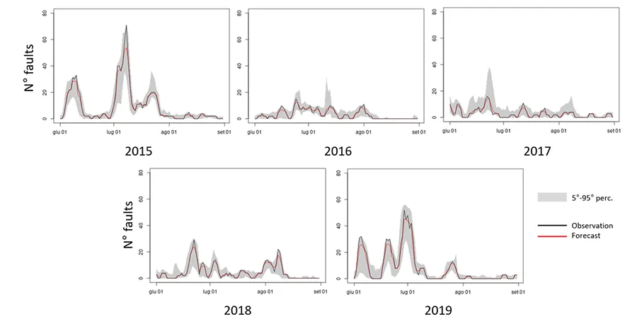
Fig. 2 reports on results of applying the model and demonstrate good correlation with observed daily fault rate for all summers. The model is also able to satisfactorily reproduce the highest peak (reached in July 2015 and 2019 when powerful heat waves affected the northern part of Italy). An indication of the uncertainty associated with the prediction is shown by the grey bands around the line of predicted faults representing 5th and 95th percentile of distribution of fault values coming from Random Forest decision trees.
Development of More Specific Resilience Assessment Approach
The model presented above is suitable to help establish the potential criticality of the cable network of an entire city with the aim of assisting the network operator in its planning of replacement investments. This approach, however, cannot pinpoint specific localized weak cable lines and give indication to the network operator about cables prone to future failure.
The following is devoted to understanding vulnerability of different types of cable joints during repeated heat waves with a view to setting up of diagnostic methods to be applied on single lines to prevent incipient faults.
Complementing Vulnerability Assessment with Laboratory Experiments
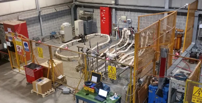
Weather and climate studies address the issue from the point of view of the threat: exogenous conditions that can influence cable system behavior and trigger cascading degradation of its components. The vulnerability of the cable systems towards this combination of stresses is a matter of technology, mounting conditions, operation, and maintenance. To address these issues, an experimental facility has been designed and realized. The final scope is to contribute to understanding the degradation mechanisms in joints and cables under the above-mentioned conditions.
Ad hoc experimental set-ups have been realized with different types of joints and cable portions. Circuit configurations were composed of cable-joint samples connected in series to form a ring in a short-circuit, where current could be injected through induction transformers with openable core to simulate daily and seasonal loading and unloading. Consequently, there are cable heating and cooling phases and where voltage was continuously applied to simulate increased dielectric stress.
Test samples were of different types, i.e. new or aged in the laboratory or in service. Different set ups in terms of cable burying conditions were simulated, as described. Each test set-up was also replicated (with the same typology of joint) by mirror rings under similar conditions but without voltage. That allowed measuring the temperature inside joints and on the surface of the conductor, using thermocouples installed in the internal layers of the joints.
A first test set-up was dedicated to situations that simulate only dry soil conditions. A second test set-up simulated cables buried directly in the ground using a soil stratigraphy in compliance with the one adopted in real service. Rainfall of different intensity and duration was simulated by means of specifically designed devices.
Sensitivity to Temperature Cycles
The first test condition simulated the behavior of cables laid underground and operated during dry and hot periods. This test was aimed at understanding the behavior and possible degradation of joints and cables under heating and cooling cycles where the soil has very low content of humidity. Daily cycles of temperature were applied to cable rings, by means of circulation of a current simulating real service conditions.
Laydown conditions under dry soil were reproduced by means of felts wrapped around the cables to simulate reduced thermal conductivity and the almost complete absence of soil humidity typical of summer periods. Thermal insulation was dimensioned to reproduce situations with a soil thermal resistivity of 2W/mK, according to the most critical conditions (as depicted in the CIGRE Technical Brochure 640).
Electrical and thermal stress was applied according to the cycles shown in Fig. 3, alternating, under applied voltage (U0 for the first 150 cycles and 1.2 U0 – 15.9kV for the remaining cycles), a heating phase, and a cooling phase of the conductor, while maintaining a minimum current circulation threshold of 100A.
Cycles from ambient to rated temperature were applied to accelerate ageing because of thermo-mechanical stresses. Maximum amplitude of the current circulated in the coils was kept within a limit of 300 A. Fig. 4 shows the resulting temperature cycles as measured on cable conductors.
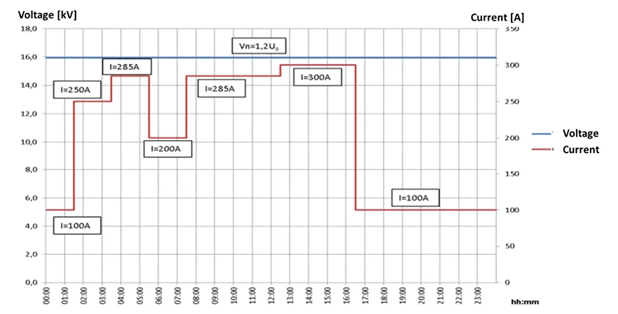
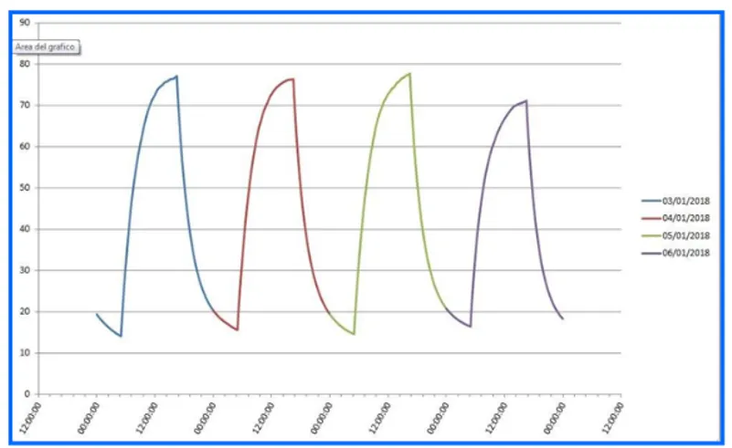
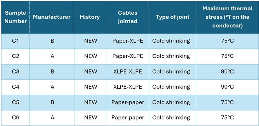
Table 2 lists the test samples used in the set-up simulating dry soil. Six new joints (2 XLPE-XLPE, 2 Oil/Paper, 2 mixed XLPE-oil/paper) from two different manufacturers (A and B) were subjected to temperature cycling under applied voltage. Fig. 5 shows the test configuration.
A total of 828 temperature cycles was applied (scoring nearly 20,000 hours of test), over more than 3 years (not continuous). Periodically, the test ring was disconnected, and the global conditions of each single cable were tested by means of partial discharge (PD) measurements, Frequency Dielectric Spectroscopy (FDS) tests and Dissipation factor (Tanδ) measurement, using commercial instruments.
The performance of different test samples revealed important influencing factors:
• Although designed to dramatically simplify mounting operation through extensive use of prefabricated sub-components, cold shrinking joints show performance that still depends on the mounting technique, skills, and precision of the operator in the trench.
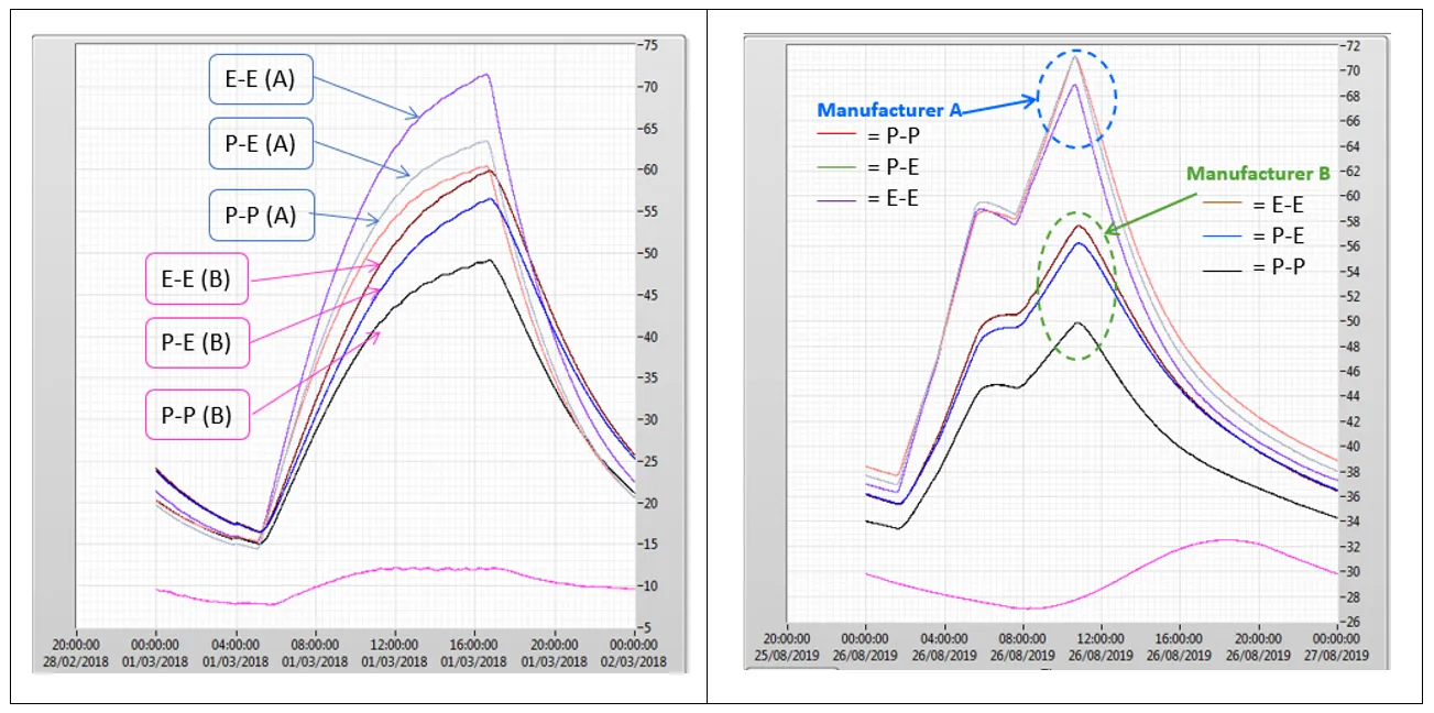
• Although all compliant with related performance Standards, temperature cycle performance of the joints depend on the manufacturer’s design solution. In fact, the materials and internal configuration can alter the capability of the joint to withstand the dielectric and thermal stresses. This fact is proven in Fig. 6, where temperature cycle plots related to samples from manufacturer A are systematically higher than those of manufacturer B. The left plot is the result of the first temperature cycle, while the right reports behavior after 500 cycles.
• Each type of joint shows a specific temperature profile: in the first cycle (new samples) the lowest temperature profiles among the samples from each manufacturer is that of Paper-Paper (P-P) joints (i.e. C5 and C6 for manufacturer B and A respectively), followed by transition joints Paper-Extruded XLPE (P-E) configuration C1, C2) and by extruded XLPE-XLPE (E-E) joints (C3, C4 respectively). This behavior is justified by safety margins adopted in the design, fit for maintaining a rated temperature lower than 75°C for paper cables and 90°C for XLPE cables.
• Thermal and electrical stresses applied during these tests can affect the condition of joints and dramatically reduce their safety margins, confirming the eventual weaknesses of materials and designs. This is shown in Fig. 6 (right): in fact, the surface temperatures of samples from manufacturer A deviate substantially from those of manufacturer B and the ageing phenomena are evident. Also, from the insulation point of view, there seems to be an influence of the dielectric stress on acceleration of ageing phenomena. Temperature plots differ between the samples under voltage and those of the unenergized ring. Moreover, detailed analysis shows a modification in the order of merit of the different joint types. In the case of Manufacturer A, characterized by a pronounced ageing, the P-P joints reach the highest temperatures, while the E-E joints remain cooler. This is a dramatic change in performance, probably linked with a rapid degradation of the paper portion of the joint: in this case the materials and configuration (manufacturer A) are weaker than expected (this change is not observed in the better performing equipment from manufacturer B).
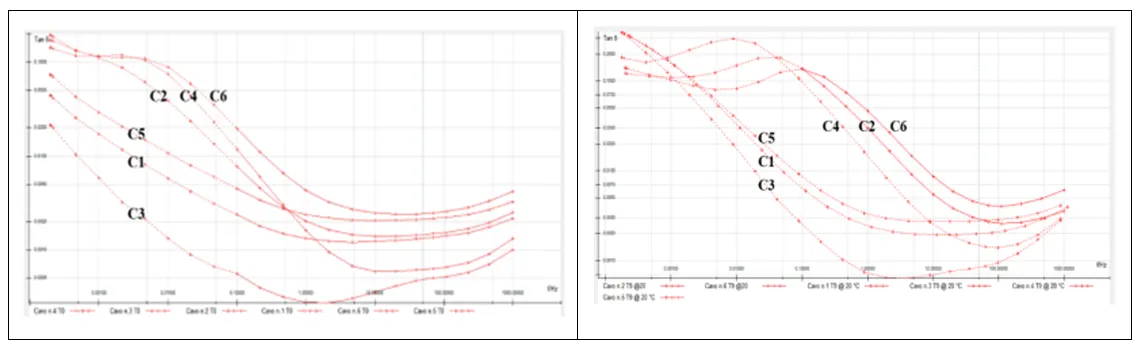
• The sole dielectric loss test at power frequency of VLF does not appear sufficient to characterize ageing, especially when extruded cables are part of the sample, since material polarization can occur from one set of testing cycles to the next. FDS measurements in the range from 0.001Hz to 5kHz allow better discriminating this phenomenon, thus avoiding biased test results and false alarms.
Use of FDS measurements carried out at regular intervals has shown the effectiveness of this methodology to assess the overall conditions of the equipment, and more specifically:
• Different designs and materials used by different manufacturers show different shapes in the FDS curves. For example, the three samples from manufacturer B show U-shaped curves (C1, C3, C5), while samples from manufacturer A show S-shaped curves (C2, C4, C6).
• While the samples age, the curves progressively shift in the upward direction and slightly modify their shape towards higher losses at each test frequency, indicating a degradation process: the shift is more evident for samples from manufacturer A with respect to manufacturer B.
Partial discharges measurements (PD) are also key diagnostic tools. The most effective way to monitor the health of the samples appeared to be the continuous measurement in contrast to the ‘off-line’ checks carried out at given time intervals.
PD monitoring was carried out through high frequency transformers clamped on the ground connection of the cables. This was able to identify progressing localized defects that were generated from the relative slip among portions of the joint: conductor, clamps, semi-conducting materials, insulation, etc. The most critical components tested showed PD activities igniting during the positive temperature gradients and unable to extinguish during the cooling down, thus showing hysteresis.
Effect of Soil Humidity
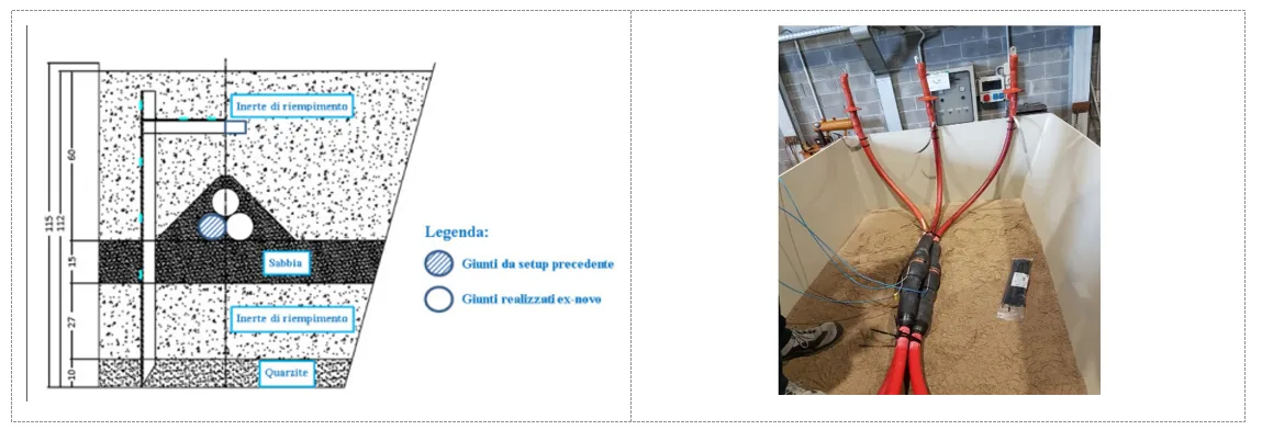
To more closely consider environmental working conditions of buried MV cables, a new set-up was realized consisting of containers filled with a layout made of different materials to reproduce the same composition, hygroscopy and granulometry as used in the field. In this test set-up, joints are positioned in a trefoil layout and adequate sensors are used to measure ground temperature and humidity, as shown in Fig. 7 (left). Test samples were composed of joints aged under dry conditions (see above) and new joints delivered and assembled from the same manufacturers as in the dry-soil test.
Designs and materials used for new samples were adapted based on results of the dry-soil sequence. Among the 12 samples tested, better overall performance of type B samples versus type A was broadly confirmed.
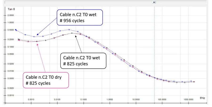
Specific attention was given to one of the four trefoils tested: the set named C2-9-10 composed of joints from manufacturer A, where C2 was aged and 9-10 were new at the beginning of the test. The first aspect considered was the effect of the presence of humidity in the soil and its possible effect on performance of the joint. FDS measurements were used to address this issue.
From Fig. 9 referred to Sample C2, the initial measurements (at T0) in dry and wet conditions are perfectly superimposable, but after 120 cycles (T1) the loss curve shifts upwards. This deviation is probably a consequence of the fact that barriers to water penetration have degraded because of the thermal and mechanical stresses introduced over the previous ageing period.
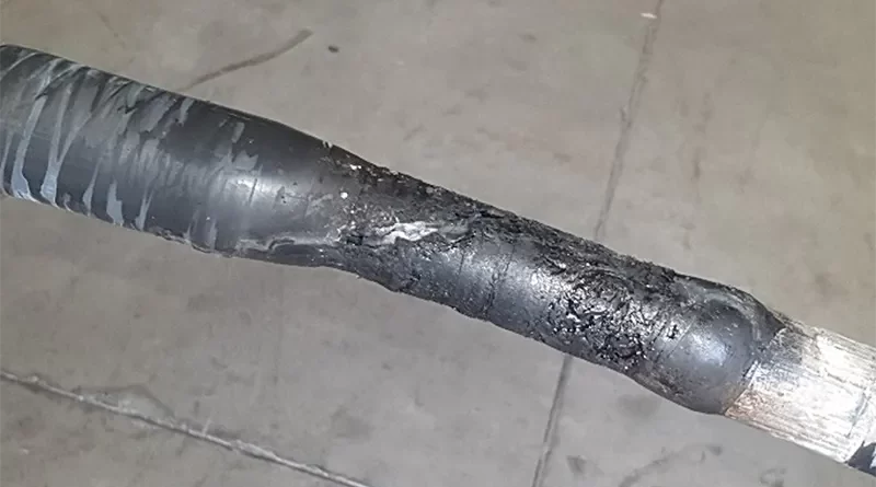
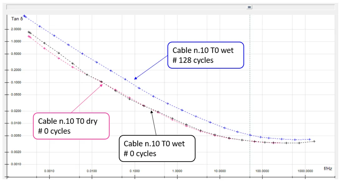
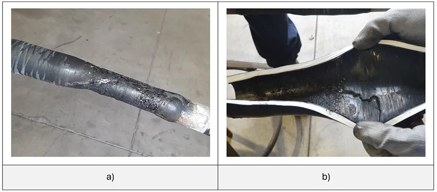
Similar phenomena occurred as well to the 2 new cable joints (9 & 10) of the same type of C2. Fig. 10, for example, reports measurements on Cable 10. In this configuration, ingress of water was apparently not linked to ageing from high temperatures (in the new set-up temperature never exceeded 50°C), but probably to a poor assembly of the joints, after the initial settling period. This problem eventually led to discharges in both new joints (9 & 10) after about 240 and 250 cycles respectively (see Fig. 11). The fault seems to have ‘wrapped’ on the cable starting from the conductor up to the screen (left); signs of discharge could also be seen along the main insulating body (right).
Presence of humidity plays an important role in dissipation of heat even if experience has shown that, in those sections of cable and in the joints subjected to thermal cycles, they also generate mechanical stresses due to different expansion coefficients which characterize the single materials used. These stresses can degrade performance of hydrostatic barriers designed to prevent moisture from entering the component.

Climate Change Scenarios Associated with Summer Heatwaves
From a planning perspective, climate change scenarios have been considered below to assess how heat wave threat can change in the future.
To this aim, an ensemble of regional climate models from the Euro-CORDEX project was used with a spatial resolution of 12 km and already widely adopted in previous studies carried out to assess the impact of climate change on the electrical energy sector. All climate models are affected from biases in 2m temperature, depending on model considered. Since the identification of potentially hazardous heat waves for the underground distribution network depends on precise temperature thresholds, it is important that this bias be reduced or removed with proper techniques and by means of reliable observational dataset. In this case observations are represented again by the MERIDA meteorological reanalysis dataset. A Quantile Mapping technique was used to perform the bias correction of 2m temperature of climate models.
The maximum reference temperature threshold for identifying heat waves was obtained by matching the temperature data from meteorological re-analysis with fault data from Italian municipalities for which these data were available. The days with a significant number of faults (greater than 5) were considered and maximum temperatures for the days in question were derived. The average between the temperatures that occurred during these days and in the various Italian municipalities for which fault data are available was about 33°C. This is therefore the temperature threshold considered for identification of potentially dangerous heat waves for underground distribution networks in urban areas.
For characterization of heat waves, the following indices were calculated:
1. Average number of events per year
This was obtained by adding up for each year the total number of events lasting at least 1 day and dividing by the total number of years in the period analyzed
2. Average duration of events
This was obtained by averaging the duration of all events in the periods considered
3. Average intensity of events
For each event, maximum deviation from the threshold (33°C) was considered and all the deviations were averaged over the periods analyzed.
These indices were obtained by considering the ensemble average of all the climate models considered in this study. In this analysis, the scenarios considered is the most pessimistic “business as usual” RCP 8.5, which indicates a scenario with no initiative to mitigate greenhouse gas emissions.
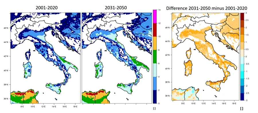
For climate change scenarios, the 20-year period 2031-2050 was considered and the variation of the 3 above mentioned indices was compared to the reference period 2001-2020. As regards average number of events per year (see Fig. 12), scenarios estimate an increase in average number of events for different areas of the Po Valley, in some areas of Tuscany. Also, especially in some areas of the center and south of Italy as well as in the major islands, where an average increase of more than 1 event per year is expected.
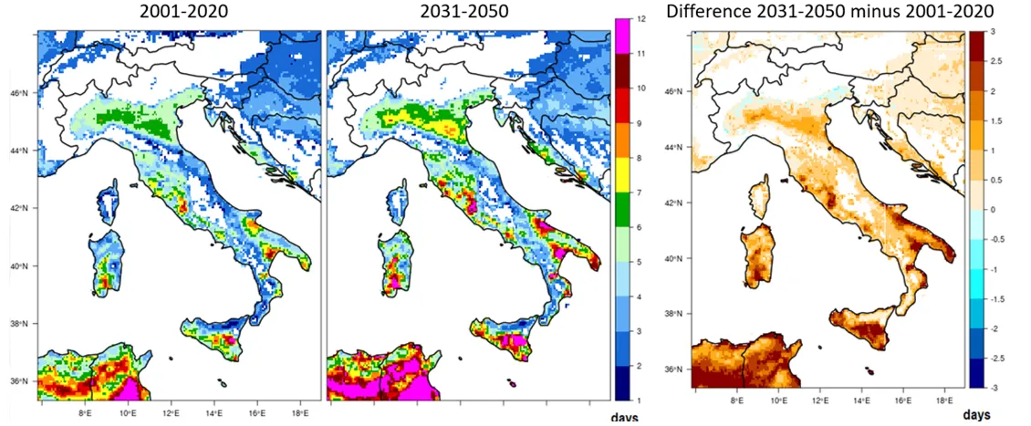
As regards the average duration of heat waves (Fig. 13), a significant increase of more than 1 day is expected on different areas of the Po Valley, while on several areas of central Italy and especially in southern Italy and islands, an increase of more than 2 days or even locally greater is expected.
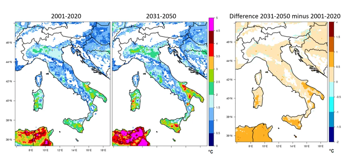
Finally, as far as average intensity of heat waves is concerned, the signal is more uniform than other indicators. A general increase of up 0.5°C is expected for the Po Valley and central Italy, while in the south (in areas such as Puglia, Sicily and Sardinia) a higher increase, i.e. between 0.5 and 1°C can be observed.
In conclusion, by mid-century, future climate scenarios show a generalized worsening of conditions associated with heat waves across many areas of Italy. An increase in number of events is expected, with corresponding higher duration and intensity: these conditions may lead to greater stress conditions on underground distribution lines in urban areas.
Conclusions & Looking to Future
Underground medium voltage cables, and more specifically cable joints, have been showing critical performance in major Italian cities under heat wave conditions. Cable joint failure rates increase rapidly during the summer when temperature and relative humidity levels become higher for longer periods in the absence of precipitation. These conditions become critical because of the concurrent pressure from high temperatures, high current flows and reduced possibility of heat dissipation through the terrain because of soil dry-out.
Correlations were found among the most important influencing parameters and an overall fault prediction model based on meteorological data and related elaborations was developed and validated. A further, more detailed, analysis has revealed that the performance of joints is also affected by their design, construction and installation parameters. Although compliant with normative requirements, a wide dispersion of actual performance is revealed by laboratory tests carried out with different temperature cycles and under humidity conditions.
In several cases, although beneficial from the heat exchange point of view, humidity can have a detrimental role when associated with presence of weak points in water seals, especially during thermal cycling. Critical conditions for cable joints are expected to increase because of climate change. Advanced models show that, in the absence of radical action to limit greenhouse gases emissions, occurrence of conditions favourable to increased stresses on underground cables will multiply in both frequency and intensity.
Research is needed along different pathways, in particular:
• A more detailed characterization of “heat wave” conditions is necessary for underground cable systems in highly urbanized and load concentrated areas, identifying more closely exogenous and endogenous variables and their thresholds, with a short-, medium- and long-term perspective.
• Identification, through conducting laboratory experiments of the electrical, mechanical, and thermal effects on underground cables and their components during the degradation process leading to potential failures under different simulated heat wave conditions.
• Testing and validation of different diagnostic indicators and techniques to be used in service and offline to characterize and prevent the progressive degradation of performances and to identify the curves of vulnerability to be used in the reliability and resilience modelling.
• Identification of methods and tools to assess the alternative measures to be adopted in the metropolitan underground networks (i.e. cables and joints replacement, extension of network meshing, use of storage systems, local flexibility services or local generator sets) to increase the system resilience and reduce Energy Not Supplied during heat wave events.
Bibliography
[1] M. Pompili, L. Calcara and S. Sangiovanni, “MV Underground Power Cable Joints Premature Failures,” in AEIT iNTERNATIONA cONFERENCE 23-25 September 2020, Virtual, 2020.
[2] K. Malmedal, C. Bates and D. Cain, “The measurement of soil thermal stability, thermal resistivity, and underground cable ampacity,” in IEEE Rural Electric Power Conference (REPC), 2014.
[3] M. Hruška, C. Clauser and R. De Doncker, “The Effect of Drying around Power Cables on the Vadose Zone Temperature,” Vadose Zone Journal , vol. 17, no. 1, 2018.
[4] S. Meregalli, S. Belvedere and S. Chiarello, “Capacità di carico di cavi interrati in funzione delle condizioni ambientali e di posa: risultati da installazione sperimentale,” Ricerca di Sistema, ERSE, no. 09004920, Milano, 2010.
[5] G. Pirovano, S. Chiarello, S. Belvedere, E. Golinelli, F. Barberis and D. Bartalesi, “Monitoraggio in laboratorio dell’influenza delle condizioni di posa sulla capacità di carico di cavi interrati e calibrazione preliminare del modello,” Ricerca di Sistema, RSE, no. 11001035, Milano, 2010.
[6] ARERA, TESTO INTEGRATO DELLA REGOLAZIONE OUTPUT-BASED DEI SERVIZI DI DISTRIBUZIONE E MISURA DELL’ENERGIA ELETTRICA, Milano: ARERA, 2020.
[7] R. Bonanno, M. Lacavalla and S. Sperati, “A new high-resolution Meteorological Reanalysis Italian Dataset: MERIDA,” Q J R Meteorol Soc, vol. 145, no. 721, pp. 1756-1779, 2019.
[8] W. Skamarock, J. Klemp and J. Dudhia, “A Description of the Advanced Research WRF Version 3,” Tech. Note NCAR/TN-475+STR, 2008.
[9] H. Hersbach, B. Bell, P. Berrisford and al., “The ERA5 global reanalysis,” Q J R Meteorol Soc, vol. 146, no. 730, pp. 1999-2049, 2020.
[10] CEI, CEI EN 60287-1-1: 2001, CEI, 2001.
[11] C. D. Peters-Lidard, E. Blackburn, X. Liang and E. F. Wood, “The Effect of Soil Thermal Conductivity Parameterization on Surface Energy Fluxes and Temperatures,” Journal of the Atmospheric Sciences , vol. 55, no. 7, 1998.
[12] L. Breiman, “Random Forest,” Machine Learning, no. 45, pp. 5-32, 2001.
[13] CIGRE, “Technical Brochure 640 : A Guide For Rating Calculations of Insulated Cables,” CIGRE, Paris, 2015.
[14] D. Jacob, J. Petersen, P. Yiou and al., “EURO-CORDEX: new high-resolution climate change projections for European impact research,” Regional Environmental Change, vol. 14, p. 563–578, 2014.
[15] L. Gudmundsson, J. B. Bremnes, J. E. Haugen and T. Engen-Skaugen, “Technical Note: Downscaling RCM precipitation to the station scale using statistical transformations – a comparison of methods,” Hydrol. Earth Syst. Sci., vol. 16, p. 3383–3390, 2012.
[16] A. Sturchio, G. Fioriti, L. Salusest, L. Calcara and M. Pompili, “Thermal Behavior of Distribution MV Underground Cables,” in AEIT International Annual Conference, 2015.
[17] T. Glickman, “Glossary of Meteorology,” American Meteorological Society, Boston, 2000.
[18] Enciclopedia Britannica, “Definition of heat wave,” 2021. [Online]. Available: https://www.britannica.com/science/heat-wave-meteorology.
[19] A. Frich, . L. Alexander, P. Della-Marta and B. Glea, “Observed coherent changes in climatic extremes during the second half of the twentieth century,” Climate Research, vol. 19, p. 193–212, 2002.
[20] Unareti, “Piano di Sviluppo 2020,” Milano, 2020.
[21] T. Bragatto, A. Cerretti, L. D’Orazio, F. Gatta, A. Geri and M. Maccioni, “Thermal Effects of Ground Faults on MV Joints and Cables,” Energies, vol. 12, 2019.
[22] M. Buhari, . V. Levi and S. K. E. Awadallah, “Modelling of Ageing Distribution Cable for Replacement Planning,” IEEE Transactions on Power Systems, vol. 31, no. 5, pp. 3996-4004, 2016.
[23] M. Kersten, “Laboratory Research for the Determination of Thermal Properties of Soils,” ACFEL Technical Report 23, University of Minnesota, Minneapolis, 1949.