This edited past contribution to INMR by Prof. Dr. Robert Ross in the Netherlands discussed the background of maintenance activities and styles in relation to Industry 4.0 and Reliability 4.0 capabilities with focus on cables and insulators.
Industry 4.0 & Reliability 4.0
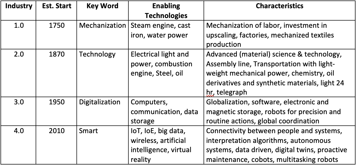
The term ‘smart’, frequently encountered for products and processes, is related to the 4th industrial revolution, dubbed Industry 4.0 and which succeeds Industry 1.0, 2.0 and 3.0 (see Table 1). Industry 4.0, and in its slipstream Reliability 4.0, concern ‘smart’ production or systems that incorporate four themes: interconnection (IoT, IoP and IoE, i.e. internet of things, people, everything); information transparency (a.o., digital twins, fusion of physical and virtual world); technical assistance (cyber physical systems (CPS), i.e., sensoring, data storage, network compatible); and decentralized decisions (algorithms and rules).
Industrial revolutions are triggered by breakthrough technologies on the one hand and societal/economic needs on the other. The roots of technologies and needs can be part of much older trends. However, through the ages, generic drives to implement technologies are factors such as adapting to crises, cost reduction, quality improvement, efficiency improvement and output increase. As an example of long trends and breakthroughs, there was already a centuries long trend of city lighting from torches, candles to lamp oil, that could be employed with the mechanical revolution.
However, only after the start of the mechanization revolution, coal gas (from 1783, Minckelers) and electrical arc light (from 1809, Davy) and light bulbs (from 1860, Swan and others) was it possible to work through the night. Steel has been produced for thousands of years yet energy-efficient and cheap mass production only became possible after 1850 (Siemens, Bessemer). This enabled compact machines that took transportation to a higher level than with steam engines. Computers, data storage and software also have been developed over thousands of years from ancient calculators, algorithms (800s), mechanical programmable devices (1800s) and libraries (writing from before 3000 BC). From about 1940, electrification of computers and semi-conductive material technology enabled compact and increasingly powerful systems that triggered the digitalization revolution.
Yet it is not only material that shapes breakthroughs; also philosophies, visions and concepts direct developments, such as computer languages and software. Massive interconnection, integration of systems and information science and technology facilitated the smart revolution. Therefore, the fifth revolution may well already be in the making but it may take decades to recognize. The beginnings of the industrial revolutions lie 120, 80 and 60 years apart, which may indicate an acceleration of revolutions. Revolutions can come with various transitions that overlap in appearance. At present, a transition to sustainability is evident but more trends are materializing. A series of ongoing trends and transitions are shaping the world of energy supply and maintenance of grids (see Table 2).
One of the characteristics associated with Industry 4.0 is proactive maintenance. The 4.0 wave capabilities enable smart maintenance. For example, the quality assurance of power electronics, systems and applications is a subject of the EU project Intelligent Reliability 4.0 (short: iRel4.0), which relates to Industry 4.0. In this project, parties collaborate along the complete value chain from wafer production to system integration. Data driven Physics of Failure models and Empirical Models are combined with Health Management and Business Processes to generate Prognostics and Health Monitoring (PHM) aiming at higher reliability at lower costs. PHM is essentially both employing power electronics in support of PHM on arbitrary systems, and applying PHM to power electronics. One of the use cases in iRel4.0 is UC-E1 that aims at a magnetic partial discharge diagnostic for cable systems, power electronic systems and associated insulators. Below is a discussion of smart maintenance with diagnostics and replacement strategies at a conceptual level so as to best understand the merits and also the limits of this approach.
Basics of Maintenance Strategy
Like other waves, e.g. Industry 4.0, Reliability 4.0 has a great impact on society and processes. The asset management of electrical grids is no exception and the perspectives are promising. But previous industrial revolutions also came with downsides and not all implementations were successful, e.g., Industry 1.0 made production more efficient but also caused unemployment and the associated costly upscaling came with financial risks and bankruptcies. It is therefore recommended to grasp the principles of maintenance not only to materialize the added value of the 4.0 revolution but also to avoid the pitfalls that may come with it. Therefore, a foundation on maintenance practice will be laid, starting with reviewing the stage of asset and system lifecycles. Next, the essentials of maintenance actions and styles are reviewed, including the impact of redundancy and repair. Finally, the integral concept of reliability centered maintenance and perspectives of smart maintenance will be discussed.
Life Stages of Assets & Systems
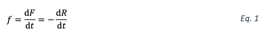
The failure behavior of product batches is characterized by a combination of statistical distributions. Each distribution can be characterized by its cumulative failure distribution function F, reliability function R, distribution density function f, or the hazard rate h=f/R. The cumulative function F(t) simply represents the fraction of the batch that failed at time t. The reliability function R (t) represents the portion that survived at t and is the complement of F, i.e. R=1-F . The density function f is the rate at which the failed fraction grows which is equivalent to the rate at which the surviving fraction declines absolutely. In mathematical terms, f is the time derivative:
Hazard rate is the rate at which the so far surviving fraction declines relatively, i.e. the probability per unit time that so far surviving products fail. This looks much like distribution density f. However, with f the decline is compared to the initial total population while, with h, the decline is relative to the remaining functioning products. In mathematical terms, f is to be divided by the surviving fraction: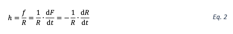
The two functions are particularly different near end-of-life of the total product batch. The surviving fraction R runs low since most products have failed and the probability of the last survivors may run up.
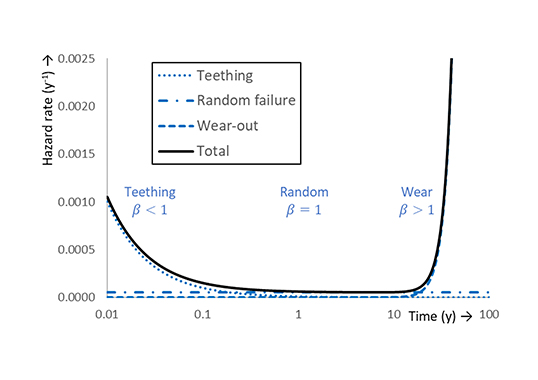
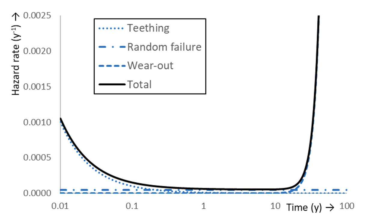
Generally, f approaches 0 while h runs up to infinity when assets wear out. The batch life cycle can be discussed conveniently by means of the hazard rate plot. Often (at least), 4 failure categories are encountered, namely teething, random, early wear and wear:
• Teething: A mechanism that often originates from production. Such a process is also called child disease or child mortality. It dominates early failures but loses importance over time. If the ruling distribution is Weibull, then the shape parameter β<1. The occurrence of such failures is commonly prevented by adequate quality control and burn-in (i.e., accelerated pre-aging). Resetting products to as good as new by maintenance has an adverse effect on the reliability. • Random failure: Any failure mechanism that is not related to operational time and ageing, thus having a constant hazard rate. Often, this kind of failure is triggered by external impact, such as digging, radiation, lightning impact, etc. If the ruling distribution is Weibull, then β=1. Occurrence of such ageing is reduced by protective measures including mechanical shields, surge arresters, etc. Except for assuring the protective measures, resetting to as good as new by maintenance, has no impact on expected life. Quality control with burn-in processes cannot prevent random failure.
• Wear: A failure mechanism related to degradation that weakens products over time. Wear leads to product end-of-life. Wear may be accelerated by enhancing the applied stress, e.g., electrical treeing with voltage and thermal ageing with current. Various laws define acceleration factors compared to a reference stress (e.g. the power law). Hazard rate increases and, if the ruling distribution is Weibull, the shape parameter β>1. If the condition can be restored to as good as new, life can then be extended. This is the basis for servicing in maintenance.
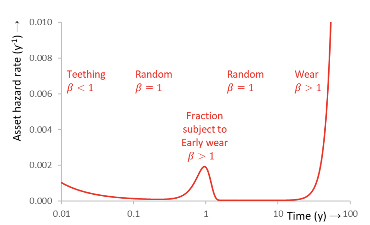
• Fast Wear or Early Wear: A type of early failures that is not teething. If encountered, it is usually deviant behavior of a fraction of the batch products due to imperfections from manufacturing, transport or installation. Early wear has an increasing hazard rate, in contrast with teething having a decreasing hazard rate. If the ruling distribution is Weibull, then the shape parameter β>1, but the scale parameter α is usually considerably smaller than normal wear. If early wear occurs repeatedly, an urgent issue may be how large the fraction of defective products is and whether repair or preventive replacement of all products is really necessary.
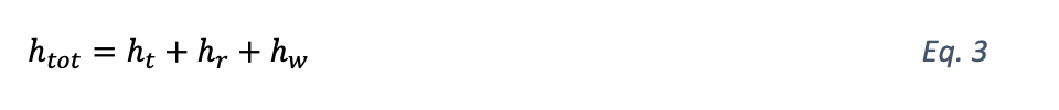
If processes compete and/or the product batch is a mix of product qualities, the failure distribution of the batch will be an entanglement of the individual distributions. If individual competing hazard rates hi are known, then the total hazard rate htot is the sum Σhj. For instance, if all products in the batch are subject to teething (with ht ), random (with hr ) and wear (with hw ) then htot (Fig. 2) is:
 This is the well-known bathtub curve. Expressions for functions and (cumulative ) are given in §2.5.1 in [4]. The momentary expected life,θ, is the inverse hazard rate: θ=htot-1 . When the product batch consists of differing fractions and the hazard rates hj of product fractions pj are known, the hazard rate hj of the mix hmix , can be given in a mathematical expression:
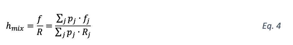
Here fj and Rj are the probability density function, respectively, reliability function of the individual processes j with j = 1,…,m. For instance, if the batch contains a fraction of defective products that suffer from early (fast) wear (with hfw) instead of normal wear, then the bathtub curve will feature a hump (Fig. 3). The height of the hump depends on size of the defective fraction. If all products are defective, then the batch is homogeneous and normal wear is completely replaced by early wear. As consequence, the bathtub curve is shortened. Momentary expected life, can be defined again as: θ = hmix-1
The main lesson from all this is that a lifecycle consists of various stages that each require a specific approach. Maintenance to rejuvenate assets and extend operational life, aims particularly at wear. It does not work for random or teething. With random processes, the auxiliary measures may require servicing to keep the constant hazard rate low. Random failure can also be reduced by better precautions such as protection, which may require maintenance. With teething, effective quality control itself may require maintenance. Extended burn-in may be considered to also eradicate early wear.
As mentioned, the teething phase is dealt with before products are supplied to the market. Testing and accelerated ageing are to ensure that the hazard rate drops to levels that are comparable to random ageing. For instance, the products in the first case, namely in Fig. 2, can be subject to enhanced stresses such that ageing in a few hours represents 0.1 year. The teething products that would otherwise fail at customers, are now taken out in the factory. The surviving products of the batch are supplied to the market and have a low hazard rate. As for customers, while the life of products starts after installation, the actual life in this example is 0.1 year longer.
Quality control may not be able to prevent early failure. In the case of Fig. 3, screening until the equivalent of 0.1 year may again prevent teething failures from entering the market. However, fast wear may not be noticeable during the screening period and may pop-up shortly after the products seem to work well. This is characteristic for any degradation process that takes time to develop (i.e. wear) but happens much earlier if products are weaker than normal.
Maintenance Activities & Styles
Maintenance consists of activities which can be employed by different styles. The 4.0 revolution can offer changes to the way activities are conducted as well as styles are implemented. Maintenance is categorized here as Inspections, Servicing and Replacement. In short:
• Inspections aim at assessing the condition of assets. The impact of the 4.0 revolution on inspections is that sensors are increasingly used to monitor asset condition. These sensors are often integrated into the asset and/or system and can communicate with a central data. Assets and systems become smart when the data is also analyzed, and feeds into the decision-making and planning of servicing and/or replacement.
• Servicing means preventive work on the asset in order to improve condition (i.e. reduce the hazard rate) and prolong the momentary expected life. With servicing, the 4.0 revolution might guide the activity by sensoring, digital twins and optimization.
• Replacement means removal of an asset and, granted the continuation of the system to which it belongs, installation of a new asset. If the system (e.g. circuit) is abandoned, replacement turns into removal of the asset and use of the space for another purpose.
Maintenance style determines planning and can be applied to most activities:
• Corrective Maintenance (CM): CM is also called run-to-fail. The concept is to not interfere with the asset condition by maintenance. This can be a rational decision and/or sometimes the only option. There is no monitoring except for checking whether the asset is still fit-for-purpose.
• Period-Based Maintenance (PBM): Also called plan-based or time-based maintenance, activities are conducted according to a planning (time, cycles, etc.) that applies to all assets alike.
• Condition-Based Maintenance (CBM): Activities are undertaken triggered by condition of the asset. Condition indicators based on diagnostics and expert rules determine necessity.
Often, Risk-based maintenance is also distinguished as a maintenance style. Risk is introduced defined as probability (hazard rate) times damage. RBM is not discussed here as separate maintenance since it will be part of the Reliability Centered Maintenance (RCM) approach (see below).
From the style descriptions, it follows that CM is reactive to malfunction. e.g. a cable joint or cable termination fails and, consequently, power supply through that cable is interrupted. This situation is to be corrected by repair. The styles PBM and CBM both interfere in order to prevent failure. The term proactive is also preventive but is used to indicate that failure cause insight, condition indicators, diagnostics and expert rules are developed, i.e. it is meant to be a more knowledgeable interference and tuned to the individual asset. But the overall aim of PBM and CBM is the same, namely the danger of failure is repeatedly reduced. In statistical terms, hazard rate is reduced or even reset.
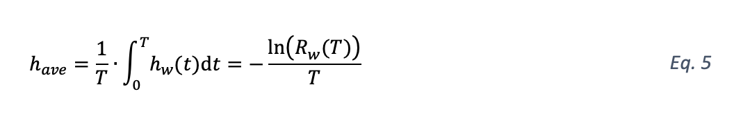
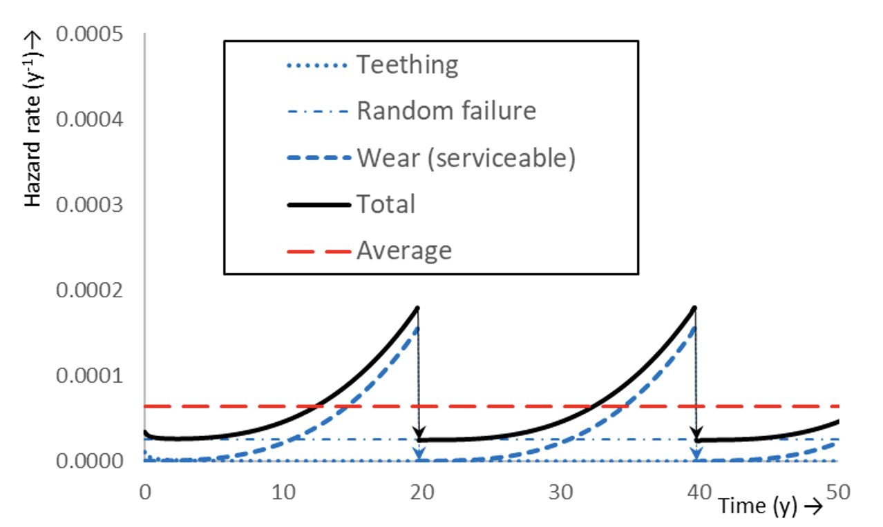
The concept of reducing hazard rate is shown in Fig. 4. With reference to Fig. 2, a part of a bathtub curve is shown due to competition of teething, random failure and wear. If wear is serviceable, then hw can be reset (ideal case). If this is done repeatedly, the bottom of the bathtub curve (Fig. 2) takes on the appearance of a sawtooth. If this sawtooth is approximated by its (running) cycle average, an elongated bathtub bottom appears, which is infinite if the reset is ideal. The average hazard rate have of wear hazard rate hw that is reset at times T (i.e., PBM approach), is found as [7]:
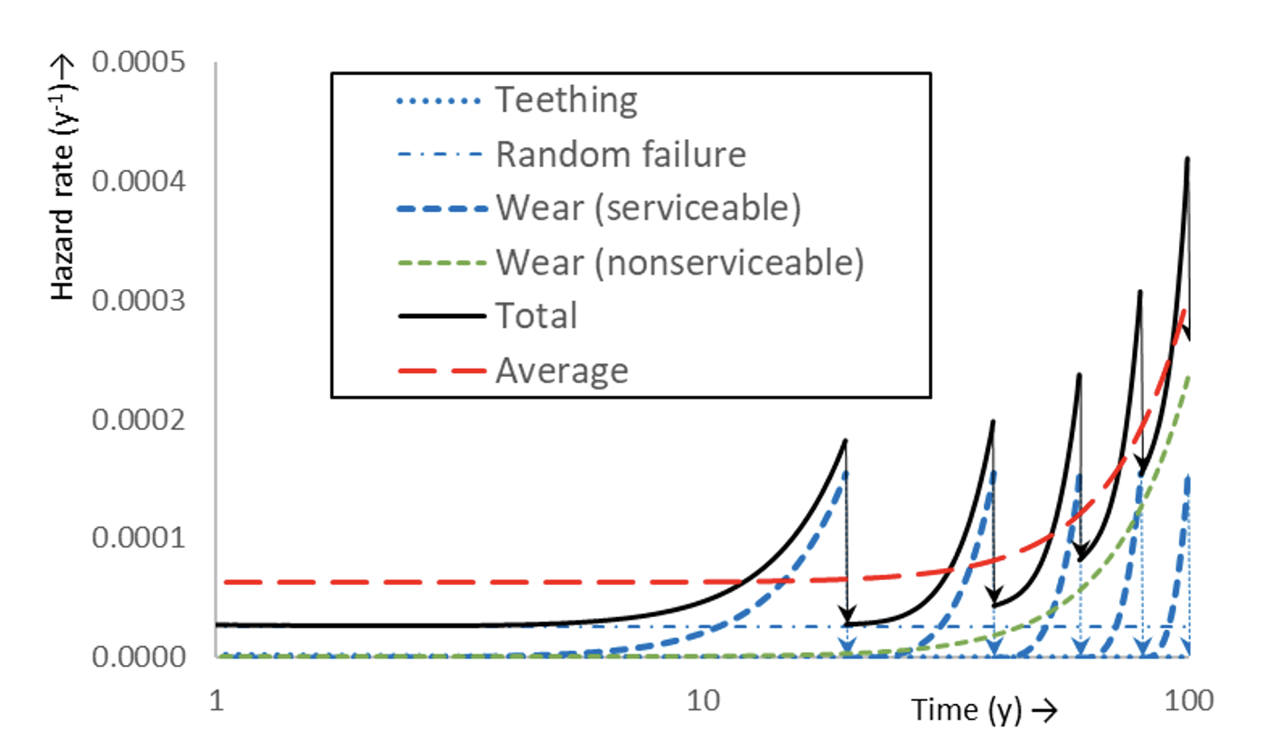
This is a constant and the actual hazard rate would fluctuate around have (see Fig. 4). However, in practice, the reset will not be perfect or not all wear is serviceable and the average hazard rate will then be increasing ultimately (Fig. 5). This restores the bathtub appearance albeit with a longer bottom than with a CM bathtub (which would be an upward continuation of the first sawtooth).
With known operational costs of maintenance activities and the capital costs (asset depreciation), the PBM cycle can be optimized [7]. The wear hazard rate and the bathtub curve apply to the whole batch which will undergo maintenance with the same cycle. If replacement is ruled by PBM, assets will be replaced after a given period irrespective of their individual condition. For some assets it may be a close call, while for other assets much operational service life may be sacrificed (cf. Fig. 6).
With CBM, this is different. It is assumed that a precursor (signal) can be detected that precedes failure. If this precursor appears sufficiently early and has a known correlation with time remaining until breakdown, it may act as an alert for imminent failure which enables prevention of the failure by e.g. servicing. CBM requires suitable diagnostics and expert rules to pick up and interpret the precursor. It is noteworthy, that the statistics to breakdown are not based on the group hazard rate (as with PBM) but rather on existence of the individually given alert and its predictive value. The latter is because the diagnostic and expert rules come with their own uncertainties and correlation with time to failure. Each individual asset will now have its own statistical distribution of failure depending on the precursor, diagnostics, expert rules and the prediction model. The overall concept of resetting hazard rate and prolonging life remains (albeit not scheduled by pre-determined cycles). CBM is tuned to the individual asset and PBM has a ‘one-size-fits-all’ approach.
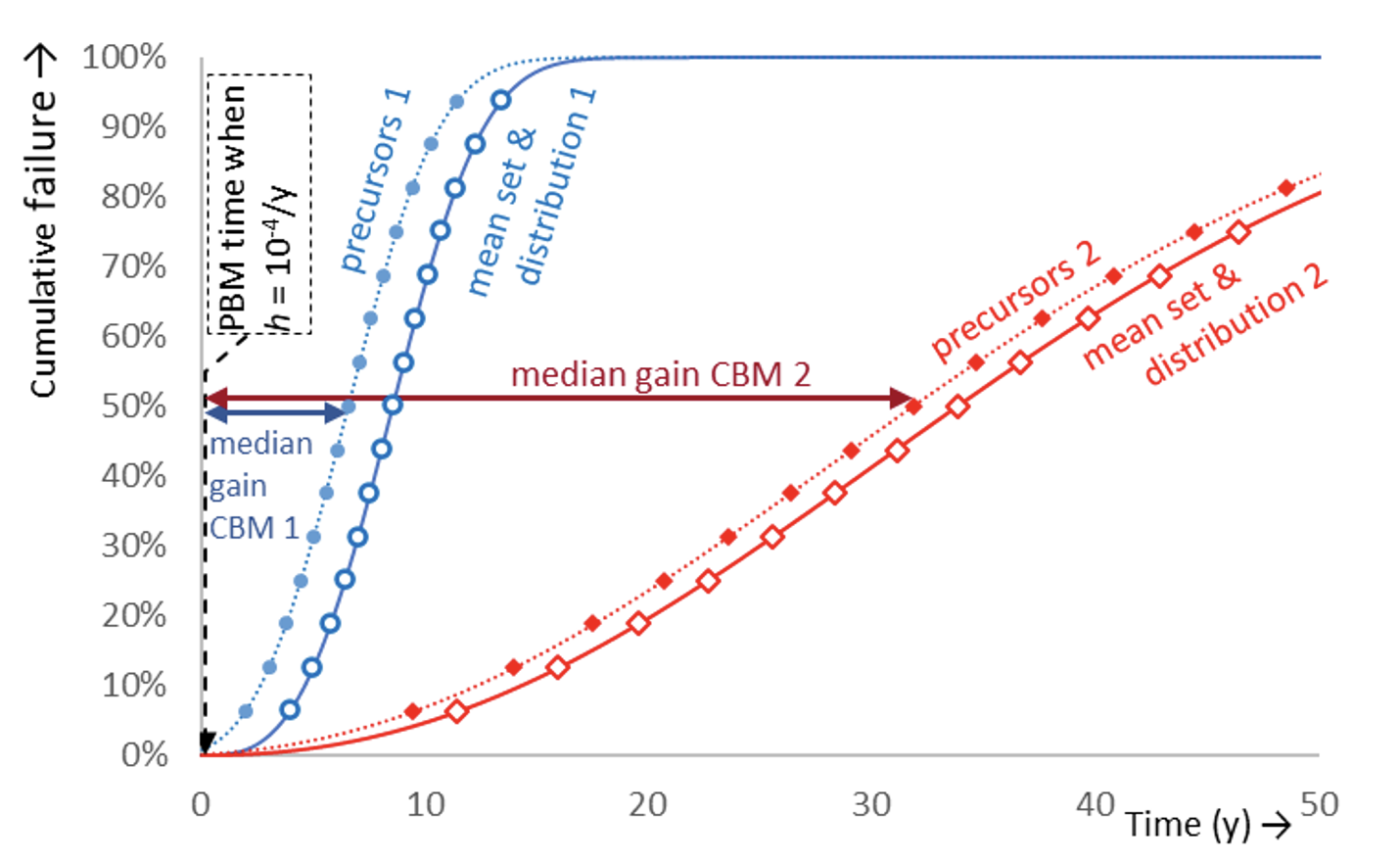
The gain of CBM over PBM tends to increase when the failure times of a group scatter more. Fig. 6 shows an example of failure behavior of two groups. This example is chosen such that PBM replacement with criterion h = 10-4/y would occur at the same time. Here, Group 1 has Weibull distribution with β1 =3.1 and Group 2 has β2 =2.2. The failure times of Group 1 scatter (much) less than of Group 2, e.g. the standard deviations are σ1 =3y respectively σ2 =17y . The median gain of CBM compared to PBM of Group 2 is about 4.8 that of Group 1. In order to be useful, a precursor should show well in advance leaving sufficient time to mitigate the imminent failure (which may be tight in Fig. 6). In the case where replacements costs would be the same, Group 2 allows more investments in diagnostics and expert rules. The steeper the failure distribution, the less gain from CBM over PBM as individuality is smaller. The intrinsic better plannability of PBM and possibly less required resources, may then be decisive. This is to be considered with decision-making about maintenance styles.

Redundancy & Repair
With either asset maintenance style, the hazard rate will still be larger than zero during operation, i.e. a certain probability of asset failure remains. To reduce the probability of discontinuity in the power supply and increase grid resilience, two important strategies are generally applied: redundancy and repair policy.
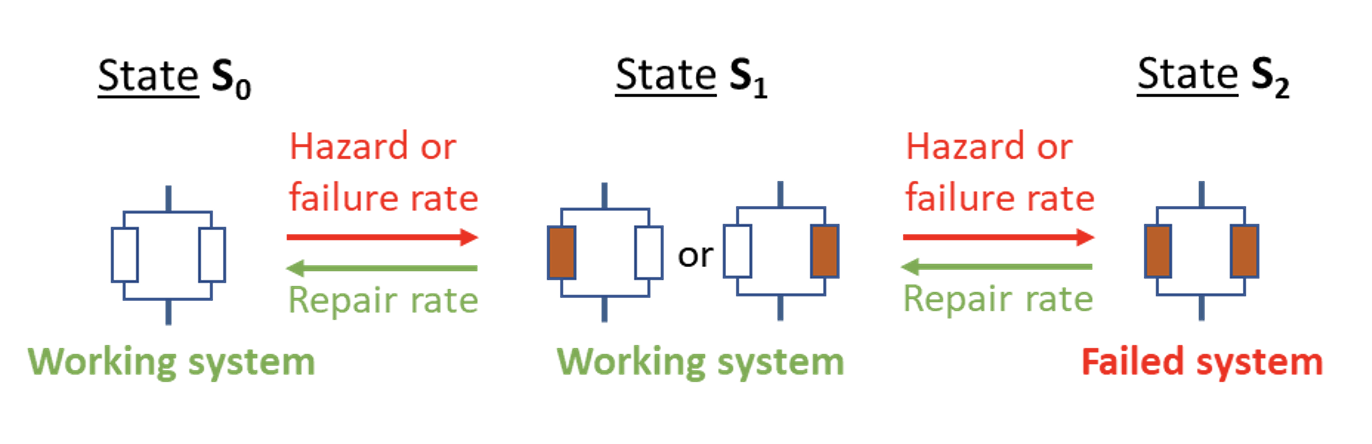
Grid redundancy means that alternative routes exist to supply electric power, e.g. a connection can consist of two parallel circuits that can each carry the full load (see Fig. 7). If one circuit fails, the connection remains in full operation and ideally even without disturbance. The connection only fails if also the second circuit fails. A triple circuit system can keep working even if two circuits fail.
The quality of assets can be expressed in terms of expected reliability and/or remaining life. For reparable assets and systems quantities such as momentary availability (A (t)), long term availability (A∞) and mean time between failures (MTBF) are often used. The availabilities A(t) and A∞ are defined as the functioning time (up time) divided by the total time, i.e. the sum of failed time (down time) and up time. The MTBF is defined as the interval between lowest repair level and the next failure. In the case of Fig. 7, if both circuits failed (State S2), a first repair would then take the system to State S1. This would mark the start of the time interval between failures, which ends when the system falls back into State S2, whether or not it has been able to return to State S0 in-between. The MTBF can be estimated with a Markov-Laplace method.
Higher order redundancy or asymmetric redundancy is also quite common. Triple circuits, emergency generators or links between distribution and transmission grids are examples. Adding redundancy increases availability and MTBF generally. Care must be taken to avoid introducing common cause failures as these can render (seeming) redundancy unreliable.
At given redundancy configuration and asset hazard rates, repair rate is an important factor for availability and MTBF. Generally, a higher repair rate improves system performance. A high repair rate is served by maintaining nearby stocks of spare parts, harmonization of technology, fast response repair teams, prepared contingency plans and protocols, etc. The achievements of Industry 4.0 with its communication capabilities and artificial intelligence should be able to contribute to adequate response. It may also serve the logistics and efficiency of CM since the performance of that style depends greatly on response to failures.
Reliability Centered Maintenance
Ultimately, the goal of an electrical infrastructure is to supply electrical energy. Regulators may define boundary conditions and targets how to operate and maintain such a grid. The EC, for instance, launched the slogan ‘affordable, secure and sustainable energy for Europe’. Such targets can have significant impact on asset management.
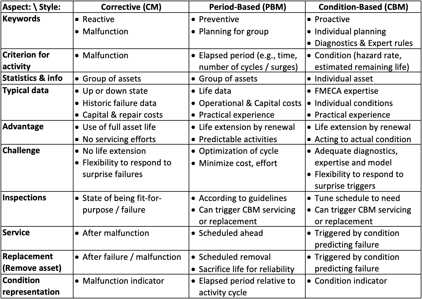
In the above, an overview of maintenance activities, maintenance styles, redundancy and repair strategies has been discussed. As shown in Table 3, the possibilities and the merits of specific maintenance styles very much depend on the assets, grid configurations, organizational capabilities and circumstances. It may be no surprise that all styles are applied in grids and for good reasons.
Reliability Centered Maintenance (RCM) is a methodology that selects appropriate maintenance approaches for all assets and (sub)systems. The mere fact that maintenance is a dedicated mix of styles also proves that neither style should be regarded superior to other styles. Often, it is about balancing 3 aspects in maintenance: performance, business, risk appetite.
• Performance is about reaching the objectives of supplying electrical energy (plus additional goals) with required quality.
• Business is about weighing options, efforts and investments against creating added value with maintenance. It involves maintainability, profit and social entrepreneurship. If two approaches deliver a similar performance, their business cases may still be very different.
• Risk is about risk appetite, knowing what mishap might occur and how it can be contained. It is not only about failing to perform and unavailability, but also about collateral damage and violation of company values like safety, and liability too. Business models may be equally attractive on average but may differ in the likelihood of unacceptable events.
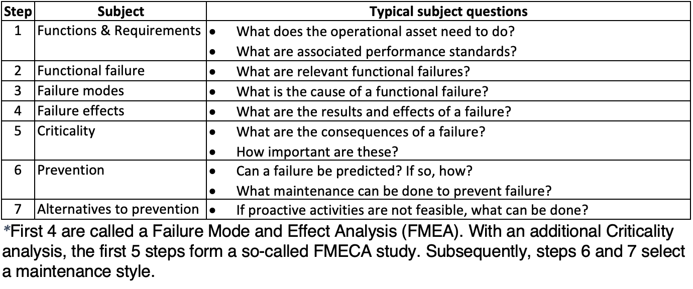
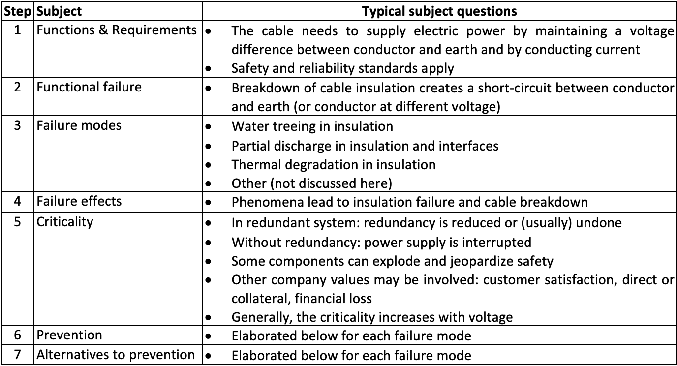
RCM originates from aerospace but has been applied to many fields. It goes through 7 steps, as shown in Table 4. A schematic representation of maintenance styles, adapted from NASA, is shown in Fig. 8.
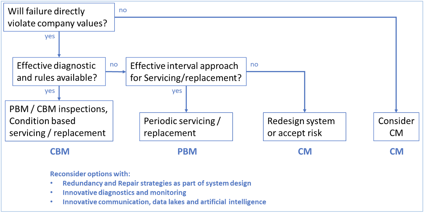

Steps 6 and 7 suggest that CBM is preferred. However, with redundancy and repair strategies in place, CM or PBM should not be discarded as lesser choices. As a domestic example, the usual high degree of lighting redundancy in a home or office plus the low costs involved for stocking spare parts (lightbulbs) and replacement, make CM a very suitable style for managing the lights. Lightbulb and LEDs are rarely replaced through a PBM scheme or CBM techniques developed to diagnose and predict malfunction of individual lamps (though where consequences are high, it might). RCM or performance-based management should be able to select CM with adequate redundancy and repair strategies. Various RCM logic trees have been developed to decide on the use of maintenance styles.
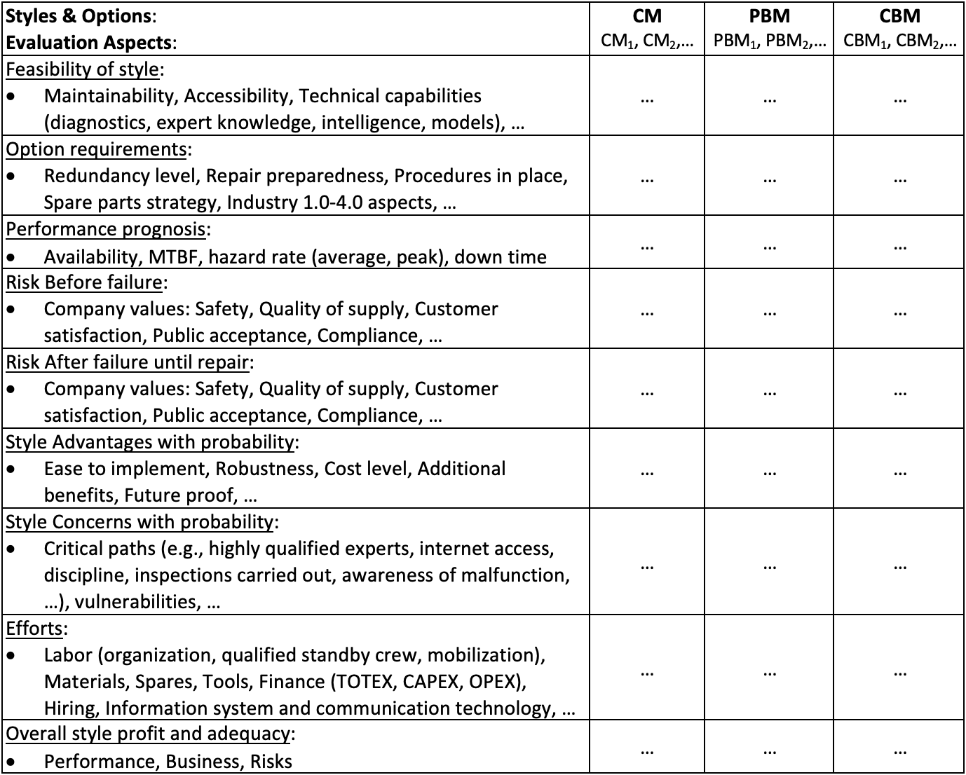
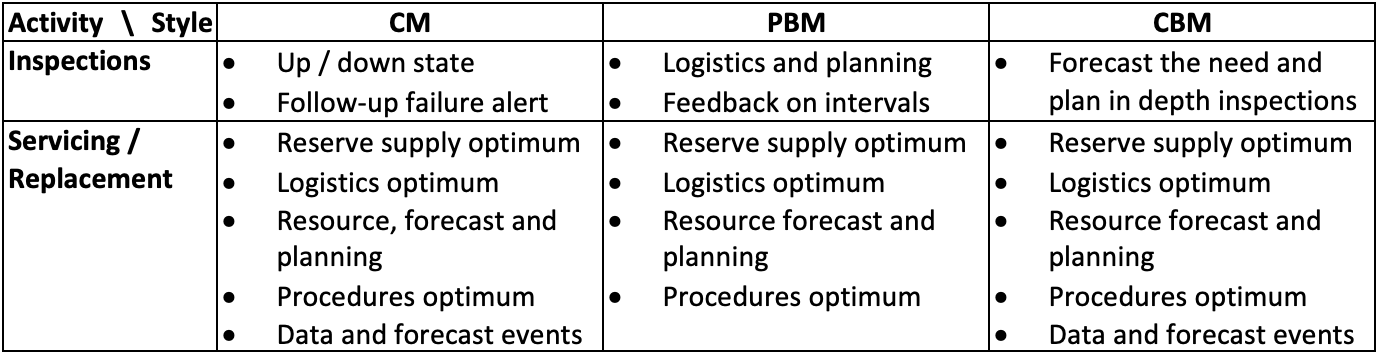
An alternative to the sequential RCM steps 6 and 7 is to evaluate the styles without prejudice (see Table 5). This provides a check on whether a style is feasible and if so, what requirements must be fulfilled. The styles can be implemented in various ways and might benefit from 4.0 wave capabilities, e.g. smart logistics for repair with CM, optimized maintenance intervals with PBM (involving costs and business values. With CBM, 4.0 wave capabilities would support critical condition prediction and trigger maintenance activities. An evaluation like in Table 5 might find the best business case. It is noteworthy, that each style can still be implemented in a CBM environment. Table 3 (last row) shows how the triggers for activities can be represented as a condition equivalent.

Perspectives of 4.0 Wave for Smart Maintenance
The Industry 4.0 and associated Reliability 4.0 wave (as per Table 1) offer capabilities that in earlier waves were either not yet available or mostly only against non-competitive costs. Maintenance that employs these capabilities, is referred to as ‘smart’. Since the 4.0 wave comprises elements of prediction, connectivity, models, AI and decision-making, smart maintenance is often associated with a next level CBM. But CM and PBM can also benefit from the 4.0 wave capabilities as discussed above. For instance, many existing underground power cable systems are not equipped with sensors and there is little servicing possible. Innovations exist that allow monitoring with respect to some phenomena, but if these are not economically feasible, the cable will be subject to CM. However, the 4.0 wave offers perspectives to the CM processes as well. For example, one challenge with CM is the flexibility to respond to failures adequately (see Table 1). Repair rate has great impact on the system availability and hazard rate. Not the asset itself but the process of CM is greatly served by response readiness, proper logistics, selecting and adapting proper procedures, handling relevant data, etc. The support of 4.0 capabilities like AI and communication offers the perspective a ‘smart CM’ that improves repair rates and therefore performance of the grid.
Likewise, 4.0 capabilities might offer the perspective of a smart PBM, that might even outperform conventional CBM. Table 5 might serve to evaluate this. Table 6 provides a non-comprehensive overview of Industry / Reliability 4.0 capabilities for maintenance activities and styles.
Smart Maintenance for Cables & Insulators
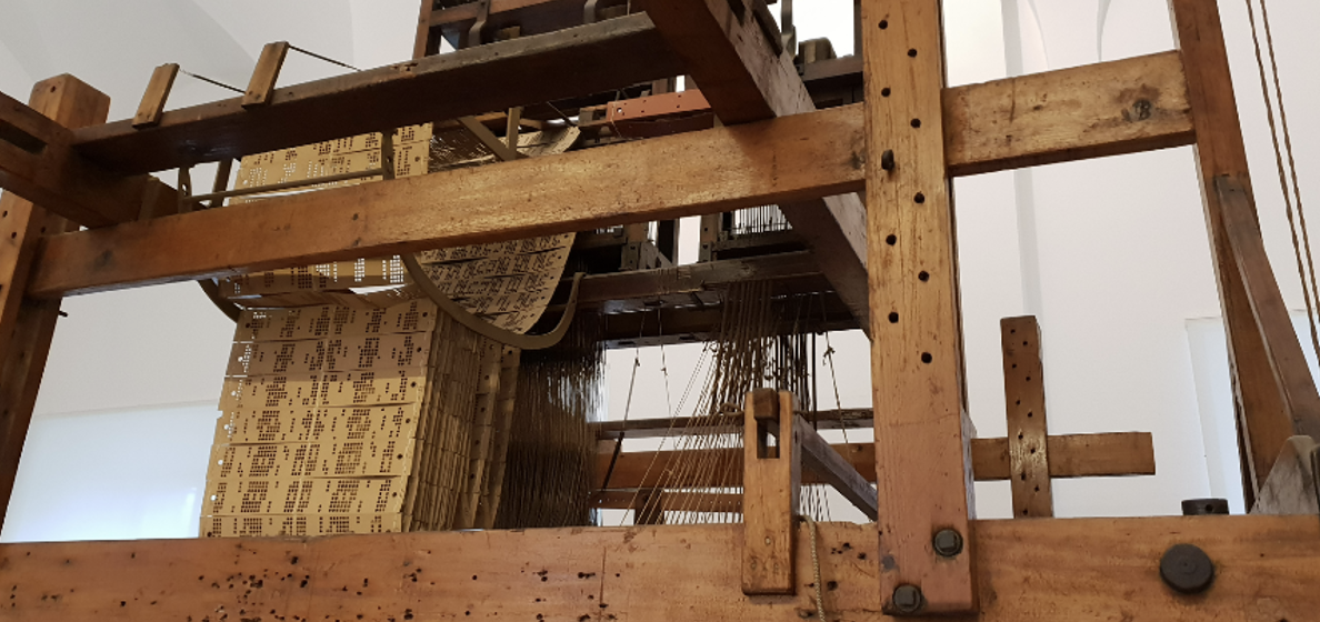
Smart maintenance can regarded as RCM benefiting from Industry / Reliability 4.0 capabilities. As in the previous section, it would not be advocated to not limit smart maintenance to a next level CBM or rigidly implement 4.0 capabilities to the full since this is not always the optimum solution. The loom with Industry 1.0 technology, shown in Fig. 1, is reported to having served well until the mid 20th century (end of Industry 2.0). It is instead recommended to remain focused on optimizing the ultimate goal, as in the EU adage ‘sustainable, secure and affordable energy supply’ or similar goals in power electronics. Overall, this focus is believed to reach more effective solutions than a rigid approach.
The following will inventory the peculiarities of cables and associated insulators with respect to failure behavior and maintenance. Next, three failure modes will be discussed as examples for RCM. The last section will touch upon miscellaneous topics such as reliability of auxiliary components.
Cables & Associated Insulators
Cables and associated insulators (terminations, connectors, bushings, joints) form cable systems. The typical cable characteristics that make maintenance challenging in some cases:
• System: often kilometers long, on land and submarine, most often (but not always) redundant;
• Technologies: oil/mass impregnated paper insulation or polymer insulation;
• Voltage: voltage levels range from low voltage (LV) 100 V, medium voltage (MV) 10-35 kV, high voltage (HV), 75-150 kV to extra high voltage (EHV) 400 kV and up;
• Life cycle: usually intended to serve 40 or more years;
• Fault effect: a single fault brings the full length to a ‘down’ state;
• Inspection: most systems cannot be inspected visually (exceptions: cables in tunnels or ducts);
• Servicing: mainly confined to replenishing oil or re-pressurizing.
As for criticality, there is a relationship between power supply and criticality. Most grids still have a hierarchical structure with a backbone of high power links for transmission over longer distances, feeding into more regional distribution networks. Higher power and longer distances with ohmic resistance conductors are served with (extra) high voltage and DC for lengths over typically 70 km (e.g., with submarine cable) to reduce ohmic losses respectively reactive current and associated losses. A fault in an (E)HV backbone link has high criticality, while a fault in a LV or MV distribution link causes much less damage (provided no exceptional violation of other company values is done). This can translate into greater fault permissibility in a distribution network than in a transmission network. This has an impact on risk appetite, need for redundancy and replacement policies. With transmission networks, it is more likely that an unacceptable risk grows without notice. Due to this higher criticality, extra redundancy and early replacement are recommended.
As for failure modes, three high impact failures are described in the following sections on RCM with the context of prevention: water treeing, partial discharge and thermal degradation.
Water Treeing
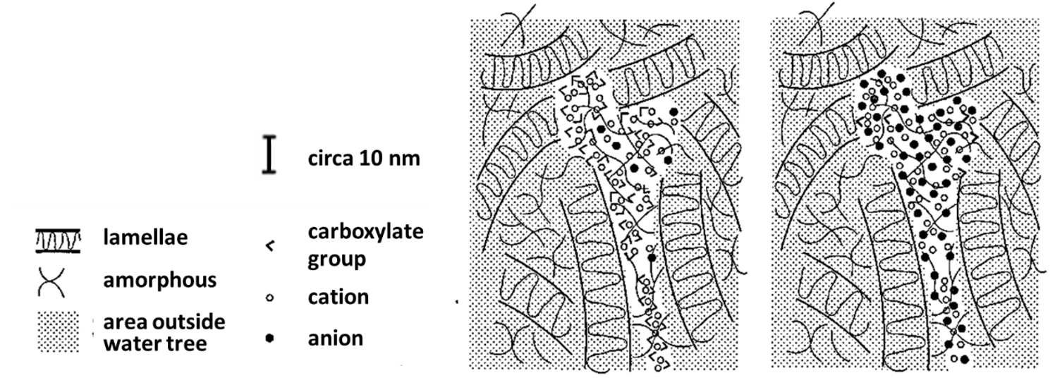
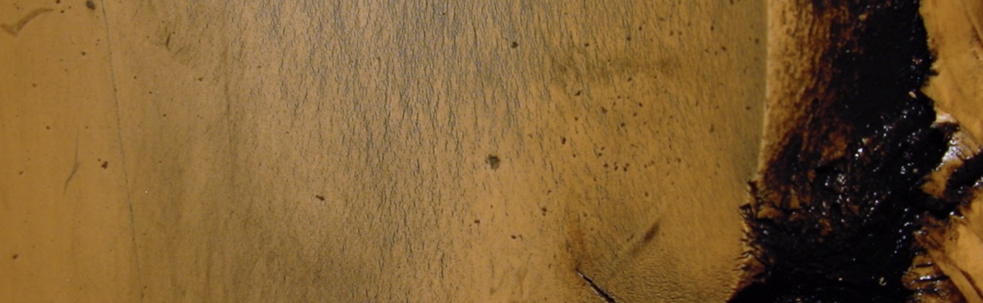
Water treeing is a degradation phenomenon in polymeric insulation of cables. It enhances the dielectric constant of the polymer by ingress of water with ions which is an energetically favorable state. This turns the insulator into an ionomer and/or polymer with tracks and pockets of trapped ions locally (see Fig. 9). A water tree is not an electric breakdown but lowers the breakdown strength with increasing length and has resulted in widespread cable failures worldwide.
Ion mobility within water trees is frequency dependent and requires sufficiently high electric fields and humidity. If a high DC field is applied to a water treed cable, the cations and anions are drawn to opposite sides of the water trees and are trapped if the external field is removed. As a result, a DC electric field inside the water tree remains. Re-energized such DC charged cables with AC, can cause enhanced electric stresses with high probability of cable failure. DC testing of suspect water treed cables is therefore strongly discouraged.
As for prevention, worldwide research into water treeing led to good insight into the degradation process. Water treeing can be significantly reduced by clean semi-conductive screens and insulation as well as keeping humidity low (prevent dissolving ions). Because of the transmitted power, HV cables represent sufficient economic value to be equipped with a fully watertight jacket, whereas MV cables in distribution usually have a MDPE jacket and are not truly watertight. For that reason, water treeing is normally only encountered with MV cables – not so much for voltage level but rather for the investment in watertight screens.
As for traditional maintenance, diagnostics was destructive. Often an unexpectedly early failure occurred, which triggered repair (CM). Then a few meter long failed piece of cable was replaced by a new piece of cable and two joints. The failed piece would be inspected visually by microscopy after staining with methylene blue, which reveals the full length of water trees if present. This could be followed up by more extensive testing sacrificing longer lengths of cable to determine the likelihood of next failures. These findings about cable condition would support decision-making about CBM replacement.
The nature of ion conductivity also offers non-destructive options to assess level of water treeing in a cable (though some consideration about many small trees versus a smaller number of big trees may be worthwhile). Characterizing ion mobility can employ the variation with electric field or frequency. Such dielectric measurements can be conducted in various ways, including spectral tan δ measurement of response analysis. Multiple parties employ tan δ measurement for water tree detection (and for water ingress in joints and indication of possible partial discharge activity).
KEPCO in Korea and Baur have developed a method that keeps track of 0.1 Hz (VLF) tan δ measurements on new XLPE insulated MV cables. An ageing index is defined based on the mean VLF tan δ and its trend. This trend consists of tan δ increasing with voltage (0.5U0, U0, 1.5U0) and with time at each test voltage. Although the model was not validated, it is reported to be based on a large set of 45,000 data points and enhanced tan δ as ion conductivity measure is highly feasible. Since the frequency and voltage deviate from power conditions, it has to be performed offline. The diagnostic will be PBM or CBM scheduled and replacement strategies will be CBM. The model is based on learning from a vast ongoing monitoring program connected to the KEPCO data base.
Some 4.0 wave elements can be recognized like connecting data from many cases to a data base, analyzing big data of many cases and building a model to capture the phenomenon. Each VLF tanδ measurement adds to the data base and the model is still under study. If a procedure could be worked out to autonomously carry out the offline VLF tanδ measurements with diagnostics and decentralized decisions, then a fully Industry 4.0 system could be produced. Whether this will be beneficial and desirable is yet to be proven. Interconnectivity and integration of data can also allow to predict replacement waves, which will assist overall replacement planning.

Partial Discharge
Partial Discharge (PD) is a long-known phenomenon that deteriorates electrical insulation. Four types of partial discharge are generally distinguished:
• Internal PD: occurring in a void within an insulation material;
• Surface PD: tracking across an insulation surface;
• Interface PD: occurring between two insulation materials, e.g. XLPE and stress control insulation in a joint or termination;
• Corona PD: from a conductor into a gas.
A PD can be viewed as an electric spark that also generates a current pulse in the conductors and produces an EM signal. PD is not a short circuit but ongoing PD can produce electrical trees, which generally disturb the electrical field locally and can ultimately lead to breakdown. Most relevant to cable systems are internal and interface PD. Nevertheless, surface and corona could occur at the terminations. PD can be detected with various techniques. There is still room for new sensing technologies since some existing parts of cable systems cannot be covered by present techniques.
As for criticality and prevention, a failure in transmission systems will violate company values more than a failure in a distribution system. However, other than quality control and proper testing, PD can occur at all voltage levels in the grid (particularly from MV and up). Considering the economic value of individual transmission links, (E)HV cable is increasingly kept under continuous surveillance. As PD can be monitored online, it is feasible to integrate PD sensing into the system operation. This also allows for monitoring trends, indicating imminent (PD driven) failures as well as to pin-pointing suspect and fault locations.
With PD, full employment is possible of the Industry / Reliability 4.0 capabilities of interconnectivity, information transparency, CPS assistance and de-centralized decision-making. Examples are the Smart Cable Guard system, Synchromerger solution and Astute HV Monitoring. Whether the investment in online PD systems is worthwhile will depend on specific situation.
Thermal Degradation
Much insulation testing concerns voltage induced ageing employing a power law. Insulation ageing can usually also be thermally accelerated. Arrhenius laws exist for both semi-steady temperatures and for cycling temperatures. Moreover, electrical insulation usually has a lower breakdown strength and a higher loss factor at high temperatures. With the trend of fossil energy being replaced by electrical energy, load on the grid is increasing, which may shorten cable lifetimes.
Thermal degradation in a mild form deteriorates the insulation over many years. However, if a cable conductor generates more heat than can be drained off through the outer cable layers and the surrounding soil, thermal instability may result. The cable temperature runs up. The resistance of an aluminum or copper conductor increases with temperature as will the losses and heat generation. This can quickly lead to thermal runaway leading to cable failure within hours.
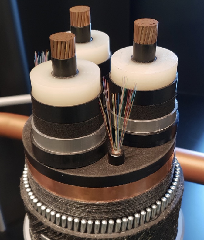
Thermal degradation can be greatly influenced by the way the power system is operated. At TenneT in the Netherlands, for example, each (HV) cable is assigned a maximum allowable current. Many cables are equipped with sensors (glass fibers) that allow monitoring of temperature distribution along the cable. With such Distributed Temperature Sensoring (DTS), the cable temperature is monitored to prevent overheating. Various DTS systems are available.
DTS systematics used to be expensive and was not embedded in system operation for all cables but rather an asset management tool to keep track of load flow through cables and the option to provide monitoring if needed. On the one hand, DTS systems and wave 4.0 capabilities have become more affordable. On the other, the stakes get higher with the energy transition and the related more intense utilization of cables.
DTS systems can therefore become much more widely implemented. Since it is an online technique, it can be incorporated employing the full 4.0 wave capabilities. But whether or not it is worth the investment and maintenance of the ICT structure needs to be evaluated.
Other Issues
Cable systems can fail by other means than the three degradation phenomena discussed above. Examples of other phenomena are: oil leakage, leaks in water tight jackets, mechanical damage by excavations, corrosion by stray currents, waxing, lightning surges, cross-bonding faults, etc. The discussion here is particularly about the generic concept of the 4.0 wave, maintenance, RCM and cable systems. This can be applied to any failure mode.
An essential element with the wave 4.0 concept is use of sensors and auxiliary systems for connectivity and data storage. Most assets in a power grid have planned lifetimes of 40 or more years. Depending on the applied grade and software, power electronics and information systems tend to have a much shorter lifetimes, e.g. about 15 years. This must be given due consideration. If a cable is attributed with a DTS glass fiber that would last 15 years, the cable would lose its thermal monitoring capabilities well before it reaches the planned wear phase. The same applies to PD sensors built into joints.
The effect of added elements in a chain is contrary to redundancy: the more elements are added to a system to function, the more links may be vulnerable and have the chain break. Redundancy is a parallel configuration, while adding elements is a series configuration. It is recommended to anticipate failures in the monitoring and communication systems or the obsoleteness of software involved. Redundancy, servicing and replacement may be required.
Finally, if an incidental cable failure has an acceptable impact with quick repair and redundancy, failure rate can become a condition indicator for a group of similar cables. This can apply to Distribution System Operators (DSOs). Recently, two DSOs were interviewed about their conception of ICT technologies in maintenance. One DSO embraced ICT and invested heavily in wave 4.0 technology and pro-active maintenance. Though it helped to anticipate failures and decide on replacement strategies, the costs of ICT and maintaining software and models were considerable. The business case is not self-evident, as discussed earlier, but must be evaluated.
The other DSO relied on rules of thumb such as a few failures per given time interval can be the reason to replace a complete group of assets. This strategy leans on high numbers of similar assets and a low hazard rate . The product is equal to the annual number of failures. In this way, can be tracked and used to detect onset of the wear-out phase – without need for advanced systems. For small groups of assets (i.e., small ), this strategy can fall short. It has been estimated that for a small group of assets in a transmission grid, may be less than 1/y, while can already have grown unacceptably large and redundancy is no longer sufficient. Particularly, for Transmission System Operators (TSOs) sensoring may be required on new HV links and, if possible, retrofits to existing links.
Discussion & Conclusions
At present, Industry 4.0 is unfolding. With it is Reliability 4.0. Characteristics for the 4.0 wave include interconnectivity, information transparency, CPS assistance and de-centralized decision-making. Although this wave answers needs in quality improvement and efficiency, it must be decided case-by-case whether expected benefits are worth the costs and effort.
Principles of maintenance were discussed in terms of activities (inspection or condition assessment; servicing or condition improvement; and replacement / removal) and styles (CM, PBM and CBM). Again, neither combination is, by definition, superior to the others. With PBM and CBM, the concept is to reset the hazard rate for wear processes. This was discussed using the bathtub model. Hazard rate reset can only be realized for wear situations that are serviceable indeed, e.g. low oil pressures in paper oil cables, gas pressure in gas pipe cable and temperature reduction with forced cooling. Replacing defective assets can be regarded as servicing of the system. Non-serviceable phenomena are water treeing and electrical treeing, once started.
As for cable systems with associated insulators, online condition assessment is not available for all failure modes. Moreover, many important failure modes (even if monitoring is feasible) are also not serviceable. But again, asset replacement may service the system. In addition to the maintenance activities, repair strategies and redundancy also play an important role in system availability, system hazard rate and mean time between failures. When evaluating system performance and maintenance scenarios, it is recommended to take repair and redundancy into account.
RCM is a method to optimize the mix of activities and styles. Optimization of the maintenance mix is to be evaluated by performance, business and risk appetite. The wave 4.0 capabilities can provide RCM outcomes that would not have been beneficial before. Though the wave 4.0 capabilities tend to be associated with CBM rather than with CM and PBM, smart CM and PBM are still thinkable and may even outperform CBM. Any style can be molded into a CBM systematic.
For cable systems, three phenomena were addressed in terms of RCM. Water treeing and PD are phenomena that cannot be serviced when it comes to the asset itself. The system can be improved by replacing affected cable circuits or suspect parts thereof. Thermal ageing is a phenomenon that greatly depends on transmitted current and thermal conductivity of the surrounding soil. Thermal damage is also likely to remain, but accumulated heat may be drained off if the current is reduced in a timely manner. Much more than water treeing and PD, thermal ageing depends on system operation (given the installation and external impacts). Water treeing is mostly diagnosed by offline tan δ measurements. PD and temperature can be monitored online and allow employing the full capabilities of the 4.0 wave. The perspectives of the 4.0 wave have in many cases materialized but wave 4.0 technology should not be applied thoughtlessly. An RCM evaluation should be performed.
References
[1] M. Hermann, T. Pentek and B. Otto, “Design Principles for Industrie 4.0 Scenarios,” in 2016 49th Hawaii International Conference on System Sciences (HICSS), Koloa, HI, USA, 2016.
[2] B. Marr, “What Everyone Must Know About Industry 4.0,” Forbes, 20 Jun 2016. [Online]. Available: https://www.forbes.com/sites/bernardmarr/2016/06/20/what-everyone-must-know-about-industry-4-0/. [Accessed 24 July 2022].
[3] iRel4.0, “iRel40 – Intelligent Reliability 4.0,” 2022. [Online]. Available: https://www.irel40.eu/. [Accessed 12 June 2022].
[4] R. Ross, Reliability Analysis for Asset Management of Electric Power Grids, Hoboken, NJ: Wiley-IEEE Press, 2019.
[5] R. Ross, “Prognostics and Health Management for Power Electronics and Electrical Power Systems,” in Proceedings 9th International Conference on Condition Monitoring and Diagnosis 2022 (CMD 2022), Kitakyushu, 2022.
[6] R. Ross, P. A. Ypma and G. Koopmans, “Weighted Linear Regression based Data Analytics for Decision Making after Early Failures,” in 10th IEEE PES Innovative Smart Grid Technologies Conference, Brisbane, 2021.
[7] R. Ross, “Health Index methodologies for decision-making on asset maintenance and replacement,” in Cigré 2017 Colloquium of Study Committees A3, B4 & D1, Winnipeg, Canada, 2017.
[8] European Commission Directorate-General for Communication, The European Union explained Energy, D. f. Communication, Ed., Brussels: Publications Office of the European Union, 2012, p. 14.
[9] European Commission, “REPowerEU: affordable, secure and sustainable energy for Europe,” Directorate-General for Communication of the European Commission, 18 May 2022. [Online]. Available: https://ec.europa.eu/info/strategy/priorities-2019-2024/european-green-deal/repowereu-affordable-secure-and-sustainable-energy-europe_en. [Accessed 20 July 2022].
[10] Wikipedia, “Reliability-centered maintenance,” Wikimedia Foundation, Inc., 2 June 2022. [Online]. Available: https://en.wikipedia.org/wiki/Reliability-centered_maintenance. [Accessed 20 July 2022].
[11] NASA, “NASA Reliability-Centered Maintenance Guide (RCM) Guide,” 9 January 2008. [Online]. Available: https://www.wbdg.org/ffc/nasa/guides-handbooks/rcm-guide. [Accessed 20 July 2022].
[12] R. Ross and P. A. Ypma, “Data analytics for decision-making about preventive replacement and incident evaluation with ageing assets,” in Cigré Colloquium SCA2/SCB2/SCD1, New Delhi, 2019.
[13] R. Ross, “Inception and propagation mechanisms of water treeing,” IEEE Transaction on Dielectrics and Electrical Insulation, vol. 5, no. 5, pp. 660-680, October 1998.
[14] E. Steennis and F. Kreuger, “Water Treeing in Polyethylene Cables,” IEEE Transactions on Electrical Insulation, vol. 25, no. 5, pp. 989-1028, 1990.
[15] R. Ross and M. Megens, “Dielectric Properties of Water Trees,” in IEEE 6th Int. Conf. on Properties and Applications of Dielectric Materials, Xian, 2000.
[16] H. Henkel, W. Kalkner and N. Muller, “Electrochemical Treeing-Strukturen In Modellkabelisolierungen Aus Thermoplastischem Oder Vernetzem Polyethylen,” Siemens Forsch.- U. Entwickl. Ber. Bd., vol. 10, no. 4, pp. 205-214., 1981.
[17] R. Ross, J. J. Smit and P. Aukema, “Staining of water trees with methylene blue explained,” in Proceedings of IEEE International Conference on Solid Dielectrics (ICSD), Sestri Levante, Italy, 1992.
[18] F. Stucki, “Dielectric Properties and I-V-Characteristics of Single Water Trees,” in Joint Workshop on Electrical Insulation & 25th Symposium on Electrical Insulation Materials, Nagoya, 1993.
[19] DNV, “Power cable diagnostics,” DNV, 2022. [Online]. Available: https://www.dnv.com/services/power-cable-diagnostics-7211. [Accessed 25 July 2022].
[20] “Cable Diagnostics,” H.V. Test, [Online]. Available: http://www.hvservices.co.za/cable-diagnostic-testing.html. [Accessed 25 July 2022].
[21] D. Kim, Y. Cho and S.-m. Kim, “A study on three dimensional assessment of the aging condition of polymeric medium voltage cables applying very low frequency (VLF) tan δ diagnostic,” IEEE Transactions on Dielectrics and Electrical Insulation, vol. 21, no. 3, pp. 940 – 947, 2014.
[22] T. Neier, J. Knauel, M. Bawart and S.-M. Kim, “A New Approach for Evaluating the Condition of Cable Systems and Estimation of Remaining Life Time of MV Underground Power Cables,” in 25th International Conference on Electricity Distribution, Madrid, 2019.
[23] Megger, “Partial discharge diagnostics,” Megger, [Online]. Available: https://uk.megger.com/products/cable-fault-test-and-diagnostics/cable-testing-and-diagnostics/partial-discharge-diagnostics. [Accessed 25 July 2022].
[24] Baur, “Cable testing and cable diagnostics,” Baur, [Online]. Available: https://www.baur.eu/en/t-and-d. [Accessed 25 July 2022].
[25] W. Rutgers, R. Ross and T. G. v. Rijn, “On-line PD detection techniques for assessment of the dielectric condition of HV components,” in IEEE 7th International Conference on Solid Dielectrics (ICSD’01), Eindhoven, 2001.
[26] DNV, “Smart Cable Guard,” DNV, [Online]. Available: https://www.dnv.com/power-renewables/services/scg/index.html. [Accessed 25 July 2022].
[27] Synaptec, “Cable condition monitoring,” Synaptec, [Online]. Available: https://synapt.ec/sectors/power-grids/cable-condition-monitoring/. [Accessed 25 July 2022].
[28] EA Technology, “Astute HV Monitoring,” EA Technology, [Online]. Available: https://eatechnology.com/sea/products/high-voltage-solutions/partial-discharge-monitoring/astute-hv-monitoring/. [Accessed 25 July 2022].
[29] W. Nelson, Accelerated Testing, John Wiley & Sons, 1990.
[30] Sensornet, “Distributed Temperature Sensing Systems & DTS Monitoring Sensors,” Sensornet, [Online]. Available: https://www.sensornet.co.uk/distributed-temperature-sensing/. [Accessed 25 July 2022].
[31] Sumitomo Electric, “Power Cable Monitoring System,” Sumitomo Electric, [Online]. Available: https://global-sei.com/power-cable-business/products/monitoring-system/. [Accessed 25 July 2022].
[32] Omnisens, “Cobra – Omnisens Securing Power Cable Integrity,” Omnisens, [Online]. Available: https://www.omnisens.com/power-cable.html. [Accessed 25 July 2022]