The decision to apply line surge arresters (LSAs) in difficult terrain is informed by estimates of local ground flash density and the ‘critical currents’ that cause flashovers. When direct stroke protection is provided using overhead groundwires (OHGW), the critical current for backflashover from grounded structure to insulated phase depends primarily on soil resistivity.

As discussed in this edited contribution to INMR by William A. Chisholm, Ehsan Azordegan and Axel Rios of Kinectrics in Canada, simplified models of lightning backflashover and transient grounding allow quantitative insight into relative performance of different treatment options. This article also offers a fascinating review of how early transmission lines were designed for lightning protection and how these designs have evolved to the present era.

---

Lightning Performance Measures & Goals

Overhead transmission line design guides devote specific chapters to mitigating shielding failures (where lightning terminates directly on an energized, insulated phase). When recommended protection systems such as overhead groundwires (OHGW) are fitted, they capture lightning strokes of both small and large peak amplitude. However, if the product of the lightning peak current and the “wave impedance” at a structure exceeds insulation strength, there may still be a flashover from structure to phase.

As the power system energy sustains this arc, a momentary fault must be cleared by other protection systems such as automatic circuit breakers or reclosers. These ‘momentary’ outages dominate the economic impact of power system reliability. A short-duration interruption of 3 to 10 power frequency cycles on a transmission line is seen as a severe voltage dip by many customers. These momentary dips lead the equipment damage costs for industrial customers with large loads that are not supported by energy storage.

Well-designed lightning protection reduces the number of momentary outages, without adding other risks of failure. Design guides rely on IEEE Standards and CIGRE references for the series of calculations made to establish the ‘shielding failure rate’ (SFR) and ‘backflashover rate’ (BFR). These terms are added to establish the total lightning outage rate, expressed in units of outages per 100 km of line length per year.

While the ground flash density (N_g, in flashes per km² per yr) varies considerably, by a factor of 1000:1 around the world, utilities tend to adapt their new overhead line designs to deliver about the same outage rates. One historical overhead line security classification includes:

• Class “C”, < 4 lightning outages per 100 km per yr
• Class “B”, < 1 lightning outage per 100 km per yr
• Class “A”, < 0.5 lightning outages per 100 km per yr

Class “A” security is a design target for ultra-high voltage (UHV) lines at system voltage  1000 kV AC. In Japan, for example, the 500 kV system achieves Class “A” security, while their 187-275 kV systems often achieve Class “B”, based on 10-year average outage rates from 1980 to 2020. With reduced insulation level (distance between arcing horns), their 110-154 kV systems achieved Class “C” security, but their 66-77 kV systems did not, during the period 1980-2010.

To improve security, considerable investment was made to improve the lightning outage rate on 66-77 kV and 110-154 kV systems. Installation of 300,000 surge arresters (LSAs) on 66 and 77 kV systems was completed in 2011, rising to 370,000 LSA in 2020 on about 38,000 km of line length. The benefits were clear. The single-circuit outage rate was cut in half, with an average of 2.1 outages per 100 km per year over the period 2011-2020, showing that it is feasible to achieve Class “C” reliability with this voltage class. When considering only double-circuit faults from lightning, all overhead transmission lines in Japan have demonstrated Class “A” reliability since 2011.

Lightning Performance: 60-69 kV Lines of 1940s & 50s

In 1955, the Ohio Brass Company (now Hubbell Power Systems) collected and published descrip¬tions of many overhead transmission lines, including those with system voltage of 60-69 kV. Each line description had tower blueprints and a list of features relevant to lightning performance, including number of days with thunder pear year (TD), positive critical lightning impulse strength (+CFO) of insulation and average annual lightning outage rate.

It is helpful to review details in this resource. Even though 60-69 kV transmission lines that delivered good service in 1955 are now obsolete, these lines may be considered for rebuilding for higher power. Physically, all lines had +CFO > 490 kV, which is considered adequate for resisting any lightning that does not terminate directly on a phase. Half of the 60-69 kV lines achieved this impulse strength with a combination of strings of porcelain insulator discs in series with wood crossarms or poles. Some lines used 10 or 11 standard 146 x 254mm discs to achieve >900 kV +CFO. Fig. 1 shows that lines with higher +CFO had lower outage rates, using an old-fashioned normalization based on TD.

Fig. 1 also shows that the 60-69 kV lines with average structure height <20 m made use of H-frame construction made from two wood poles and a single crossarm. Median span length with wood H-frame structures in Fig. 1 was 168m, compared to 234m for steel lattice structures.

In 1955, the utility industry relied on meteorological station measurements of TD to normalize performance against local lightning activity. With the data provided, it was possible to estimate a ‘critical current’ I_crit for backflashover (kA) from the provided values of lightning impulse strength (kV), average footing resistance (Ω) and factors accounting for parallel overhead groundwires on shielded lines. Fig. 2 shows a rough downward trend in normalized outage rate as I_crit increases.

When the critical current I_crit > 200 kA, it is often considered ‘lightning proof’. Fig. 2 shows good performance for two of the three 60-69 kV lines with I_crit  > 200 kA and the majority of the 60-69 kV lines achieved at least Class-C security.

Lightning Performance, 60-69 kV Lines Upgraded by 1955

It is interesting to review the measures adopted to improve lightning outage rate of 60-69 kV lines before 1955. These measures are described below to aid in visualizing the parameters in a simplified model for the peak magnitude of the first negative return stroke (RS) that causes a fault.

Negative Shield Angle

When OHGW are placed directly above or outboard of phase conductors, they offer better protection than configurations where the OHGW spacing is less than the horizontal phase-to-phase spacing. The 66 kV line of the Philadelphia Electric Company operated for 37 years with the shielding configuration shown in Fig. 3.
Each of the OHGW extends 8’ (2.44m) from the central lattice structure. The top-phase conductors of each circuit are spaced 5.5’ (1.68m) when the insulators are vertical. Shielding angle here is negative (-16), as the top phases are tucked inside of the protection zone of the OHGW. Shielding angle to the middle phases is 0 since the OHGW on each side is directly above. This line is thus considered well shielded.

With +CFO = 650 kV from 8-disc strings of 127 x 254 mm (spacing x diameter), this line achieved a lightning fault rate of 0.9 per 100 km per year, giving Class B security in a region with an average TD = 31.7 days per year. For future reference, the “Coupling Coefficient” C_n to the top-phase conductors was 0.44. If the OHGW voltage is 1000 kV, the phase voltage will become 440 kV and the voltage across the insulation will be (1000 – 440 = 560 kV). This factor reduced stress on insulators and improved lightning performance. When more OHGW are present and they are close to the phases, the value of C_n increases.

As the middle and bottom phases in Fig. 3 are farther from the OHGW and their mutual surge coupling coefficients are, respectively, 0.35 and 0.29. The role of the coupling factor in backflashover calculations is developed further in other INMR references and shows how impulse corona effects increase Cn beyond its easily calculated geometric value.

Insulator Grading Rings

Grading rings are fitted to polymer insulators to improve service life and used to mitigate damage from power system arcs. It seems the engineers at Cincinnati Gas & Electric wanted to evaluate the merits of corona rings in 1938, by fitting them at each end of the ceramic disc insulator strings on Line 1061, as in Fig. 4. These rings at line and ground end were not used on the insulators of Line 1062 on the left, which was completed 10 years later.

With average footing resistance R_f=2.3 Ω and +CFO = 945 kV, neither of the 66 kV circuits in Fig. 4 had any lightning faults despite a high local value of TD = 51.4 days per year in Cincinnati. Part of the good performance of this line may also be attributed to its use of negative shield angles, -8 on Line 1062 and -7 on Line 1061 to accommodate the extra length of the grading rings (8’ – 6’ 5.25” or 470 mm). However, as an introduction to estimating the critical current concept, it would require a lightning surge of 410 kA flowing in 2.3 Ω to generate a surge voltage of 945 kV. This is a low-probability event, as lines with critical current >200 kA are generally considered ‘lightning proof’.

Sacrificial Low Voltage Circuit

The drawing in Fig. 5 shows a single-pole construction with a single OHGW at the top of the pole, providing a typical +30 shield angle to the top two phases. The line description notes that the fourth conductor is one phase of a 12/6.9 kV distribution system that is using the OHGW as a neutral.

When lightning terminates on this line, even with low footing resistance of R_f=4 Ω, the median RS current of 30 kA would generate a 120 kV impulse voltage that will backflash from pole to the distribution circuit. Its lightning performance will be poor, but every time the distribution circuit faults to ground, it protects the transmission circuit by raising the coupling coefficients in Table 1.

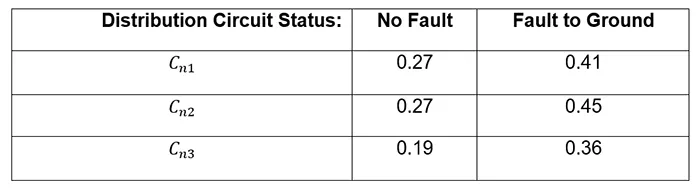
When the distribution line faults to ground, there is a large improvement in C_n3 in Table 1 for the bottom phase of the 67 kV line, which is at the same height as the distribution line. This height is the crossover level between an “underbuilt” GW (located below all the phases) and an “embedded” GW (located above one or more phase). The benefits of underbuilt and embedded GW for 345-kV double circuit lightning performance, including effects of corona, are found in IEEE Standard 1243, Fig. 9.

With a modest TD level of 28 days/year, the line in Fig. 5 achieved Class-C reliability with 2.0 lightning outages per 100 km per year. While Fig. 5 shows that only 5 standard discs were used in suspension, the +CFO was increased to 1100 kV by using unbonded crossarms with 1.7m wood path.

Underbuilt Groundwire (UBGW)

Poor lightning performance in the 1930s of the Duquesne Light Company 69 kV ring lines surrounding Pittsburgh led to rebuilding in 1941-42 that variously:

1. Added a peak to the tower top to raise the single OHGW, providing reduced shielding angles of 19 to 25°;
2. Installed an underbuilt groundwire (aerial counterpoise) to increase the coupling effect;
3. Reduced the tower footing resistance below 25 Ω, with average value 10 Ω, using short radial counterpoise and additional vertical ground rods;
4. Increased the insulation strength from +CFO = 610 kV with six standard discs to:
a. 1030 kV by replacing steel arms with dual-member 5’ (1.52 m) wood arms, or
b. 1025 kV by using eleven discs

Fig. 6 shows the dual-member wood arms and location of the UBGW for a rebuilt line that achieved Class-C security of 2 outages per 100 km per year in a region with TD=44 days/year.

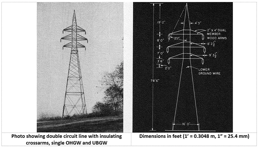
The location of the UBGW in Fig. 6, in concert with the elevated single OHGW, may have been optimized to deliver the same computed values of C_n≅0.33 at all 6 phase conductors.

Lightning Performance of Modern 60-77 kV Lines

The innovative use of externally gapped line arresters (EGLAs) as well as current-limiting arcing horns (CLAH) on 66 kV and 77 kV systems in Japan has been well documented in INMR. A 2021 CIGRE guide provides additional details of utility experience with TLSA. Recently, the discussions of IEC Standard 60099-11 have covering applications of LSA on overhead lines. This group has designated the CLAH technology generically as a type of ‘Surge Arc Suppressor’ (SAS).

When an LSA conducts surge current, it converts the protected phase to a GW that provides strong increases in C_n on nearby unprotected phases. This develops the possibility of using two different voltages on the same structure and achieving good lightning performance by applying LSA only to the lower-voltage system.

Simplified Model of Backflashover

The calculations of I_crit have been introduced using a crude estimate of the insulation strength (+CFO, kV) divided by the low-frequency footing resistance R_f (Ω). The estimate is improved by considering surge impedance coupling coefficients, that effectively increase +CFO by a factor of 1\/(1-C_n ). Other factors are combined in this section to develop an accessible model that gives insight, rather than numbers. Every aspect of the simple model here has been improved.

Simplified Backflashover Models based on Fixed Ramp Time of 2 μs

Backflashover calculations use parameters of the first negative return stroke (RS), because these have the largest values of I_pk that tend to give the highest levels of insulator voltage V_pk.

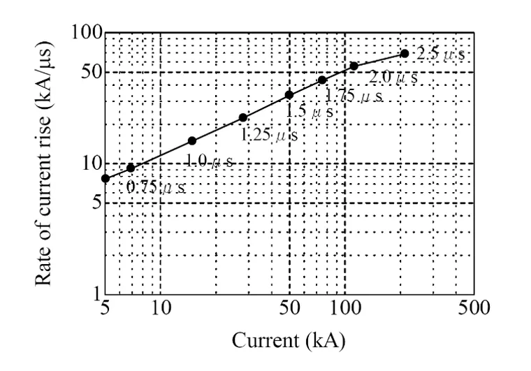
Choice of a linear ramp wave with zero to peak time of 2 microseconds (2 μs) is a standard, simple way to evaluate the overvoltage from peak current >100 kA in Fig. 7 that are high enough to cause backflashovers. The simplified model, and its inversion to establish critical current I_crit (kA) from the insulator positive lightning impulse flashover voltage U_50 tm  (kV), are found in Equation 1.

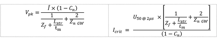
where:
• C_n, the surge impedance coupling factor from nnoverhead groundwires to the phase (dimensionless);
• n, the number of groundwires including OHGW, UBGW, neutrals, messenger cables and any phases protected by operation of LSAs (integer);
• Z_{n GW}, the surge impedance of the groundwires in parallel in one direction away from the structure, considering self-impedance Z_ii and mutual impedance Z_ij (W);
• Z_f, the impedance of the stricken tower footing and earthing system to remote earth (W);
• L_str, the inductance of the stricken tower segment (μH), established by product of travel time to earth times average section surge impedance;
• U_{50 @ 2μs}, the critical lightning impulse flashover from the volt-time curve (kV), usually evaluated at the ramp wave crest of 2 μs and adjusted for span length using a volt-time curve.

When the zero-to-100% rise time is fixed, at t_m=2μs or another value, it is used to convert any path inductance to additional voltage rise above the footing potential rise, using the model ΔV=L dI/dt=L×I/t_m. The total voltage rise at tower top is the structure current flow I multiplied by the sum Z_f+L_str/t_m. The voltage rise at intermediate positions relative to tower base is established by the structure current flow and the inductance from those points to the ground, again converted to V/A using a fixed ramp time t_m.

There is no single value for I_pk. Instead, it is described by a log-normal statistical distribution, with median 31 kA and standard deviation of ln(I_pk) between 0.48 and 0.66. The tower footing impedance Z_f in Equation 1 also has a log-normal distribution. The log standard deviation of resistivity, based on 300m distance between sites, has been found to be in the range of 0.9 for regions in the U.s. and Portugal. The distribution of V_pk, computed using Equation 1 is thus the product of two, very wide statistical distributions. Failure is always an option, and engineering is done instead to a desired failure rate specification, such as the Class A/B/C reliability requirements.

Subsequent strokes have lower median values of I_pk (12 kA versus 31 kA for first RS) and faster rate of rise (S_m=40 kA/μs subsequent stroke RS versus S_m=24 kA/μs for first RS). The equivalent linear waveform duration, defined by t_m=I_pk /S_m is t_m=0.31 μs for subsequent strokes and t_m=1.28 μs for first RS. The question of whether subsequent strokes can cause backflashovers is open because it is difficult to establish the insulation strength test data needed for steep-front waves. This discussion assumes that subsequent strokes do not cause backflashovers – but also adopts a model that subsequent strokes will guarantee a fault for every shielding failure from a first RS with low peak current.

Simplified Backflashover Models Based on Fixed Ramp Time of 1.8-2.5 s
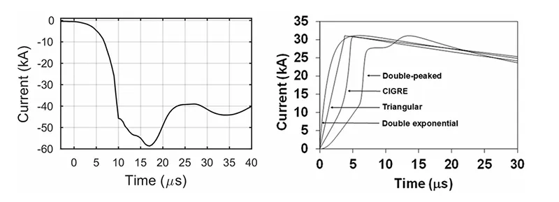
Observations of lightning surge currents on 500-kV towers in Japan noted a modest increase in peak current (PEAK) after the “First Peak”, shown by “PEAK-1” in Fig. 8.

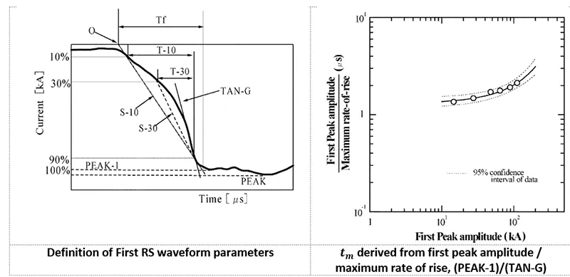
The equivalent ramp front time, extrapolating back from first peak at the rate of S_max to zero current, seems to increase slowly in the range of 1.8 to 2.5 μs, depending on peak current magnitude.

Usually, the insulation strength is well known, relying on test results such as those in Fig. 9 so the process is inverted to compute the critical peak value I_crit that equates V_pk with this strength. This is done for the expected range of values of Z_f. Then, the probability of receiving a first return stroke exceeding I_crit is established by inverting its log-normal distribution, using a LOGNORM.DIST function in a spreadsheet or a log-logistic estimate P(i>I_crit)=1/(1+(I_crit/31 kA)^2.6 ).

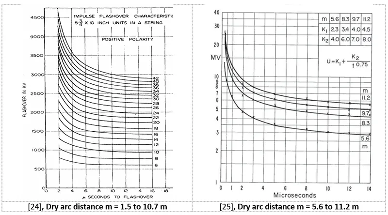
In 1997, IEEE adopted a hybrid approach, where a fixed 2 μs ramp current is assumed, but a variable time, based on the span length, is used evaluate the insulation strength with a generic volt-time curve, as in Fig. 9. The argument was that the backflashover voltage wave deviates downward from the standard double-exponential 1.2/50 test wave at the time that reflected voltage waves from adjacent structures, so that if flashover has not occurred at that time, it will not occur at all. The curves in Fig. 9 are generalized for insulator strings 1 < m ≤ 11.2m as V_fo= m ×(400+710t^(-0.75) ) where flashover voltage V_fo is in kV and m is in meters.

Simplified Backflashover Model Based on Ramp Times of 2, 4, 6 μs

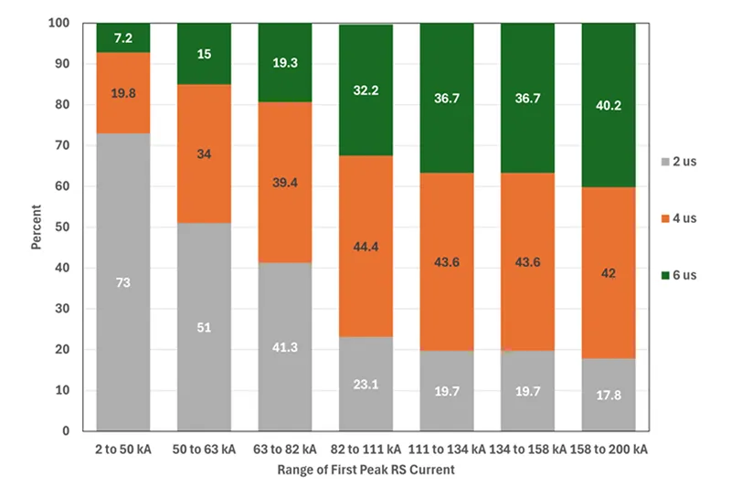
Discussion of the appropriate ramp time in simplified calculations has been underway for at least eighty years. Movement away from a purely resistive model, incorporating structure inductance L with a ramp current, is featured in a 1956 paper.

A resource on UHV lightning performance side-stepped the question about the “best” ramp wave by selecting randomly among 2, 4 and 6 μs with a Monte-Carlo parameter selection program. The fraction of surges with each value of t_m was defined by Clayton and Young in 1964. The fractions with each ramp time varied from 73% with t_m=2 μs for peak current < 50 kA, up to 40% with t_m=6 μs for I_pk>158 kA in Fig. 10.

With the use of data from lightning location systems, Udo endorsed use of t_m=4 μs for explaining the lightning performance of tall 500-kV double circuit lines, mostly with m = 3.8 m clearance between insulator arcing horns. With the assumed median 420m span length, the return of reflections from adjacent structures in Fig. 11 would appear in at 2.8 μs.

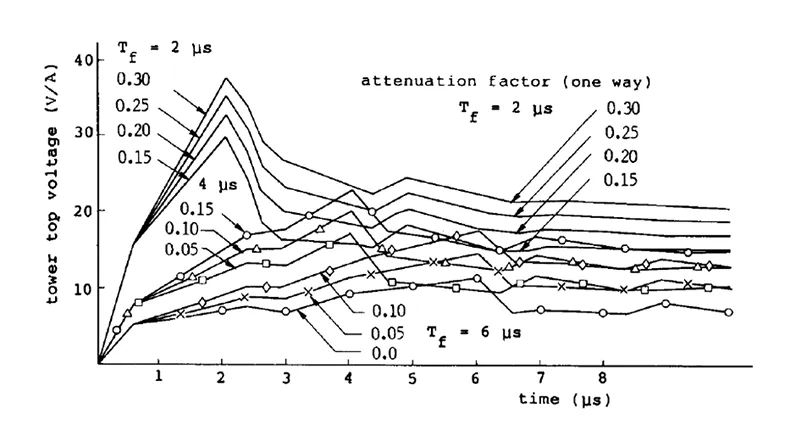
The peak tower-top voltage with t_m=2 μs in Fig. 11 is nearly twice the value for t_m=4-6 μs. This highlights that smaller, faster values of t_m emphasize effects of tower inductance (surge impedance times travel time) while larger, slower values of t_m give overvoltages that depend on footing resistance and span length.

Improvements to Simplified Backflashover Model
In addition to questions about representation with a single, fixed ramp waveshape rather than using variable t_m that changes slowly with increasing I_pk, previous INMR tutorials and many other references describe several adjustments to the simple model in Equation 1.
• The volt-time curve for impulse flashover, shown in Fig. 9 which can be extended for nonstandard waveshapes using integration methods;
• The surge impedance coupling from those OHGW, faulted and arrester-protected conductors that carry a fraction of the lightning surge current in each direction from tower top;
• The additional voltage rise associated with fast-rising current flow in the inductance of a thin monopole structure;
• The variability of soil resistivity and footing impedance from structure to structure;
• The effects of corona, which absorbs energy from the lightning and reduces stress on the insulators;
• The effects of line voltage, as one phase will always have an instantaneous voltage that adds to the stress;
• The effects of line surge arresters on the distribution circuit, which convert protected phases to extra groundwires and thus provide some benefits even to the unprotected transmission phases above.

Some highly detailed models, with advanced electromagnetic response of structures as well as nonstandard insulation strength, evaluated the critical current using a concave wavefront with fixed Td₃₀ time of 3.8 μs from I₃₀ to I₉₀ compared to than a ramp of 2 μs from 0 to peak I₁₀₀. Fig. 12 shows the limitations of the ramp (triangular) waveshape in representing an observation.

Among all these modeling factors, uncertainty as to the value of soil resistivity and its direct effect on structure resistance is the most important aspect of a representative backflashover outage rate calculation based on a critical first RS current.

Grounding

The flow of lightning surge and fault current into the system of OHGW and footings depends on several factors, each with some uncertainty. The main factors are:
• The soil resistivity ρ(Ωm) which in geotechnical reports may be expressed as conductivity κ (mS\/m);
• The distance around the outside of the foundations, which is an initial approximation to the effective perimeter P(m) of the equivalent hemisphere;
• The local footing resistance R_f (Ω)=ρ/P;
• The series inductance of OHGW connections to adjacent spans and of any long, horizontal buried wire (counterpoise) components; and
• The frequency, which may be fixed (50 or 60 Hz) or may consist of a spectrum to model an impulsive waveshape like lightning.

Equation 1 shows that calculation of I_crit backflashover threat depends largely on the footing impedance Z_f. For many years, utilities have assumed that Z_f≅R_f, the low-frequency resistance that is measured by isolating the structure from any OHGW. Arguments continue about whether the influence of high-current ionization expands the size of the electrode, or whether the soil itself has frequency-dependent parameters [30]. While ionization is significant for a singe rod in the earth, it has little calculated influence on the size of a grounding system consisting of lattice tower foundations and tests are not feasible. For this reason, simple models for soil ionization should not be applied to transmission line backflashover calculations. In contrast, frequency-dependent soil parameters can be evaluated with the test methods described below and provide appropriate adjustments for the relation between Z_f and R_f in both frequency and time domain.
It is easier to visualize the effects of lightning surges in the time domain using the simplified model in Equation 1 than in the frequency domain. All the earthing that receives and dissipates lightning currents within t_m will be useful. Any part of a grounding system that exceeds the “effective length” l_eff and does not participate in absorbing surge current has limited benefit.

A process to establish grounding parameters and footing impedance Z_f is illustrated with results from a recent field campaign along a shielded 69-kV transmission line in a high-altitude region of high resistivity.

Theory: Relating Soil Resistivity to Footing Impedance

General Model for Rf of Any Electrode
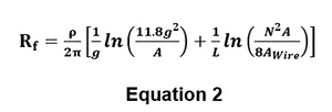
The resistance of a wire-frame approximation to a solid ground electrode can be split into two terms, one (Geometric resistance) related to the overall shape and size with a shape factor, and an added term (Contact resistance) to correct for the incomplete fill factor. Equation 2 shows that both terms depend linearly on ρ.

Where geometric radius

where r_x,y,z are the radial dimensions of the electrode (m) measured from its center, A is the overall surface area of the electrode (m²), L is the total length of wire (m) and wire surface A_wire is L x  2π r for wire radius (m). The value of N corrects for mutual coupling when a number of wires extend out from a point.

To use Equation 2 well, we need estimates of ρ in the volume of soil around each structure. This is an area of rapid progress in remote sensing, especially to provide the fraction of clay content in depth 0-2 m as well as estimates of depth to bedrock of the soil. For existing structures, it is convenient to use the structure itself as an electrode, rather than to carry out resistivity surveys at some distance away and hope that the remote values match those nearby.

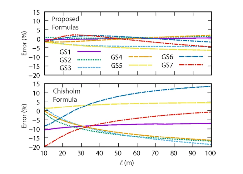
Recently, a series of papers evaluated a set of seven different counterpoise configurations to manage Z_f. The configuration “GS5” in Fig. 13 is common in many countries, notably France and Brazil. Generally, the overall length l is increased in higher resistivity soil, up to the point where it achieves no further benefit under lightning surge conditions. Whether horizontal or vertical, a good estimate of this maximum effective length l_eff=√(ρ×t_m ) with resistivity ρ (Ωm) and ramp rise time t_m=2μs in our simplified model. The role of l_eff is shown in Fig. 13 for a calculation with ρ=750 Ωm, t_m=2.5 μs, l_eff=43 m. Once the counterpoise length exceeds 43 m, the impedance in Fig. 13 does not change from its asymptotic value of about 9.5 Ω even though the power frequency resistance R(l) continues to fall.

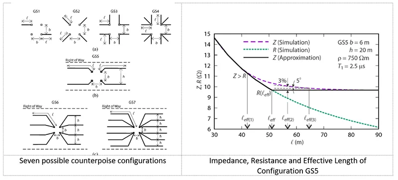
The work includes equations that describe the low-frequency resistance of each electrode in Fig. 13. A comparison was made from these individual expressions to the results from a general expression Equation 2. Fig. 14 shows that the agreement for the four-leg counterpoise electrode GS5 is excellent (difference < 5%) while results for wires extending radially from each leg (GS2, GS3 and GS4) disagree by more than 10% when l > 30 m.

Numerical Models
Massive foundations are required for some of the T-Pylons in the United Kingdom, consisting of a dense cage of steel rebar (up to 10 x 10 m) supplemented by up to 16 vertical driven piles. The effective perimeters of four such foundations were computed using CDEGS, a standard numerical model.

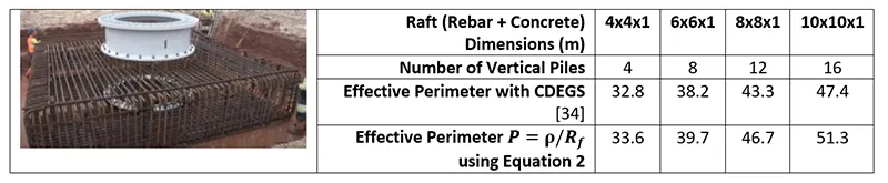
As was the case for individual electrode models GS1 to GS7, the agreement between the CDEGS model results in Table 2 and the simple Equation 2 is satisfactory.

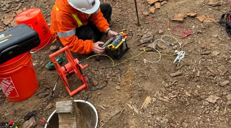
Grounding Test Program Location & Motivation

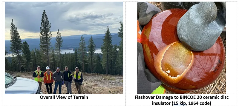
Preliminary studies matched observed fault times on a 69-kV overhead line to the times, locations and peak radiated fields of lightning strokes. Data from five years were reviewed, and it was concluded that most of the faults were caused by large-amplitude strokes, leading to backflashovers. The high-altitude region in western USA shown in Fig. 15 had low ground flash density. Flashovers during infrequent lightning storms sometimes led to suspension disc glaze damage such as that seen the same figure.

One option for improved lightning performance, considered a last resort based on component count and electrical clearances, was to rebuild the tower heads and fit line surge arresters across every insulator. A field test program to measure grounding parameters R_f, Z_f and ρ(t) from power frequency up to lightning impulse was undertaken to develop alternative remediation strategies.

This work used several different techniques and instruments, including directional testing of R_f with four Rogowski coils (41 to 5078 Hz) and Zed-method testing of Z_f in the time domain (100-1500 ns) on seven selected structures. Near each tested structure, conventional Wenner resistivity surveys at power frequency were complemented by step-wave tests on a buried hemisphere to give ρ(t) from 10 ns to 1 s, covering 8 decades of frequency spectrum. Descriptions of these test methods are found in the recently revised IEEE Standard 81-2025 which was approved in June 2025.

Wenner Resistivity Survey

The Wenner method for soil resistivity measurements from 1915 remains in today’s standards as a configuration of four, equally spaced probes. When the two outer probes are energized, a potential difference between the inner probes appears. The ratio of inner probe potential to outer probe current gives a resistance value that is converted to an apparent resistivity. From reciprocity, when the excitation and voltage connections are interchanged, the earth resistance tester should show the same reading, and when it does not, there is a measurement problem such as high probe resistance or crossed connection. Fig. 16 shows a typical Wenner probe array with small spacing.

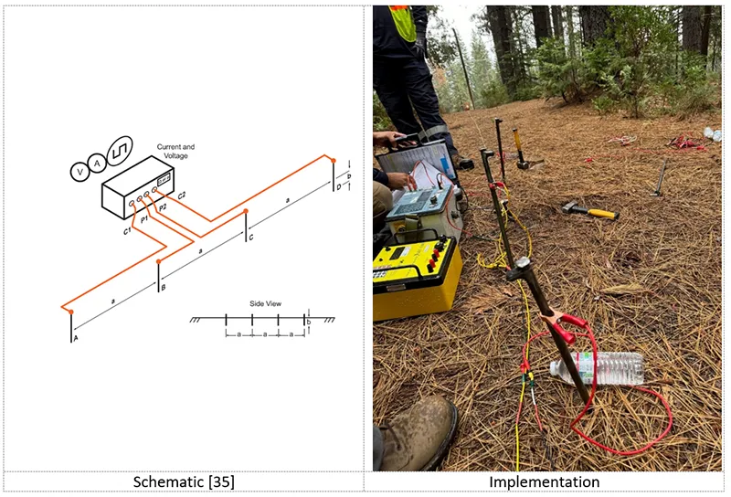
The team in this survey work used bottles of tap water to moisten the soil and reduce each test probe resistance. At some locations, to obtain enough test current, two or more probes were connected in parallel. In locations with high soil resistivity, getting adequate test current to satisfy the programmed requirements of an earth resistance tester can be a time-consuming and frustrating process.

Some utilities take a Wenner measurement for a single probe spacing, perhaps 20 m, and count on the corresponding soil depth to be about 15% of this spacing, 3 m. It is a better practice to take readings at several different probe spacings and to evaluate whether the soil is “layered” with different resistivity at different depth. The use of more than four probes (for example 32 simultaneously) to develop 2-D soil tomography is feasible but not widely used in electric utilities.

Fig. 17 illustrates another limitation of a Wenner survey (or other tomography) of soil resistivity. The survey line must be located at some distance from the right-of-way to avoid interference at power frequency and also to mitigate the possibility that the line has been equipped with counterpoise.

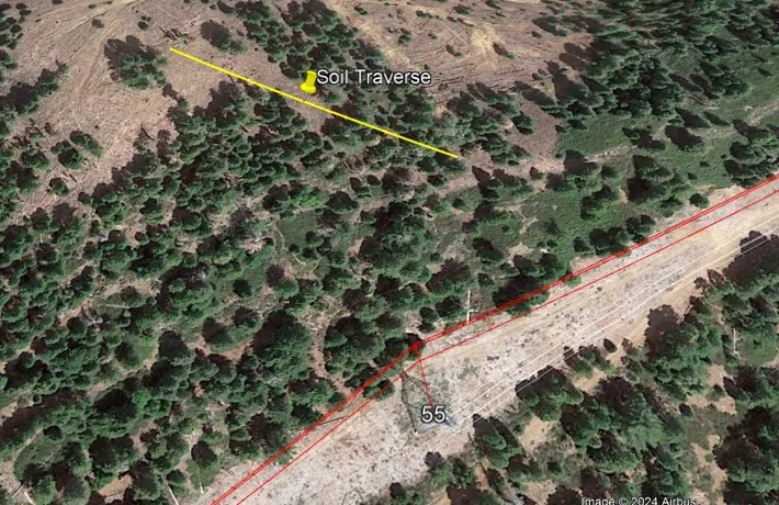
There is no guarantee that the soil properties measured along the traverse are the same as those in a soil volume centered at the structure. If civil engineers have been involved in tower spotting, they have most likely selected the areas of strong, dense rock and rejected locations with soft clay.

After the resistance readings have been recorded for each probe spacing, IEEE Standard 81 describes a standard analysis method. A formula is given for the apparent resistivity, which corrects for the probe length. Then, Fig. 18 shows a spreadsheet plot of the data, with apparent resistivity on the vertical axis and probe spacing on the horizontal axis, both using logarithmic scales.

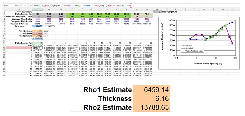
The Standard 81 Annex A provides an infinite-series sum of the apparent resistivity associated with two-layer soil with upper layer ρ₁ (Ωm), layer thickness d(m) and basement layer ρ₂ (Ωm) to infinite depth. This is based on the reflection coefficient K between the layers and the probe spacing. The spreadsheet in Fig. 18 implements the equations. The “Solver” function is used to minimize the squared difference between the ρ_a values computed from field data, and the ρ_a values that correspond to the two-layer soil model parameters. When we consider the field data for spacing of 3 to 30 m, the soil model suggests an upper layer of 6500 Ωm with depth 6 m over a basement layer of 14,000 Ωm, with appropriate rounding to two decimal places.

The two-layer soil model is adjusted to fit the Wenner test results for probe spacing of 3 to 30 m. For closer spacing, the results are not relevant to calculating resistance of large electrodes, such as four pier foundations, each steel-reinforced concrete with 3.2 m depth and 0.9 m diameter and spaced on the corners of a 25’ (7.6 m) square footprint. However, these values are more relevant to electrical safety calculations as they influence the foot-to-soil resistance.

The test results in Fig. 18 show a decrease in apparent resistivity for probe spacing of 50 and 70 m. This can be fitted with a three- or four-layer soil model than also requires numerical methods to evaluate the resistance, rather than equations implemented in a spreadsheet. However, this moves the process far away from “simplified”.

Transient Resistivity Using Hemisphere & Oblique Method

An alternative for measuring soil properties was defined by CIGRE as shown in Fig. 19.

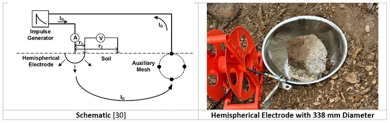
Generally, an impulse generator impresses a current into the metal bowl, and the potential difference from the bowl to the nearby soil at distance r₂ is recorded at the same time on an oscilloscope. When the potential difference is taken at 90º to the current lead, the influence from the auxiliary mesh at the bowl and voltage probe are equal, so they cancel out. This leaves a resistance reading that increases with 1/r₂. Equation 3 gives the resistivity estimate at each distance in uniform (but frequency dependent) soil as:

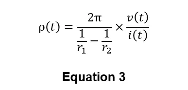
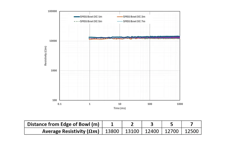
For this field campaign, the bowl radius r₁=0.169 m and distance from the edge of the bowl varied from 1 to 7 m, giving 1.169 ≤r₂ ≤7.169 m.

The hemisphere tests used the Oblique Test Method to establish resistance and resistivity simultaneously. When the potentials are measured along a curve that maintains the same distance CP to distance EP in Fig. 20, two terms in the calculation of surface potential cancel, so the resulting impedance rises as the inverse of distance EP. Resistivity is the slope of this ΔZ/Δ(1/X) relation, multiplied by a factor of -2 π. The intercept of the plot of z(t) versus 1/X in Fig. 20 is the impedance at infinite distance, identical to the value obtained for the in-line configuration with EP at 61.8% of the distance EC.

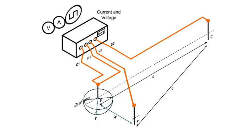
The quality control loop in Oblique-method transient measurements using earth resistance testers and transient signals is closed by computing the effective perimeter P(t)=ρ(t)/Z(t). As the bowl size is constant, we expect P(t)=2πr₁ for all values of time. Additional description of the equations behind the Oblique method are found in the recently revised IEEE Standard 81-2025.

Oblique Test on Hemisphere: Results with 1s Pulse
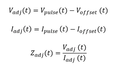
An on-off switch was used to excite the bowl relative to a remote connection to ground. The current and voltage to points on the earth nearby were sampled. Then, the corrections for offset in Equation 4 were applied to give V_adj (t) and I_adj (t) in Fig. 21.

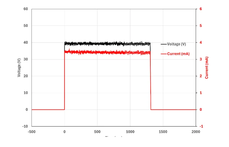
The values of Z_adj (t) were converted to ρ(t) using Equation 3. There is a slight trend to lower values of ρ(t) with increasing distance in Fig. 22.

Oblique Test on Hemisphere: Results with 30 μs & 5 μs Pulses
The hemisphere resistivity test was repeated with pulse generators with faster rise and fall times. One had duration of 5 μs, and its open circuit voltage of 225 V impressed a current as high as 600 mA on each transition in Fig. 23. The other pulse generator had 500 V output, slower rise time, longer duration and higher average impressed current.

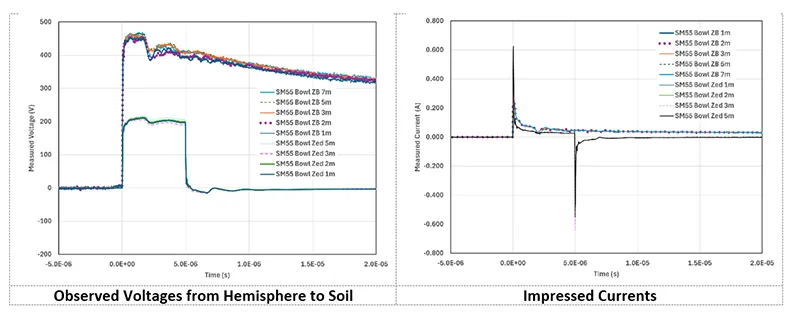
With both pulse excitations in Fig. 23, there is a reduction in voltage and current at 1.7 μs. This corresponds to the back-and-forth travel time of the 152 m current reaction lead (CRL) to the “auxiliary mesh” remote ground in Fig. 19.

The resistivity was interpreted for each distance and pulse shape using Equation 4, then Equation 3. Unlike the values for ρ(t) from 1 to 1000 ms in Fig. 22, there is a pronounced rise in Fig. 25 from 2000 Ωm @ 0.1 μs up to 9000 Ωm @ 5 μs and leveling off at 10,700 Ωm @ 30 μs.

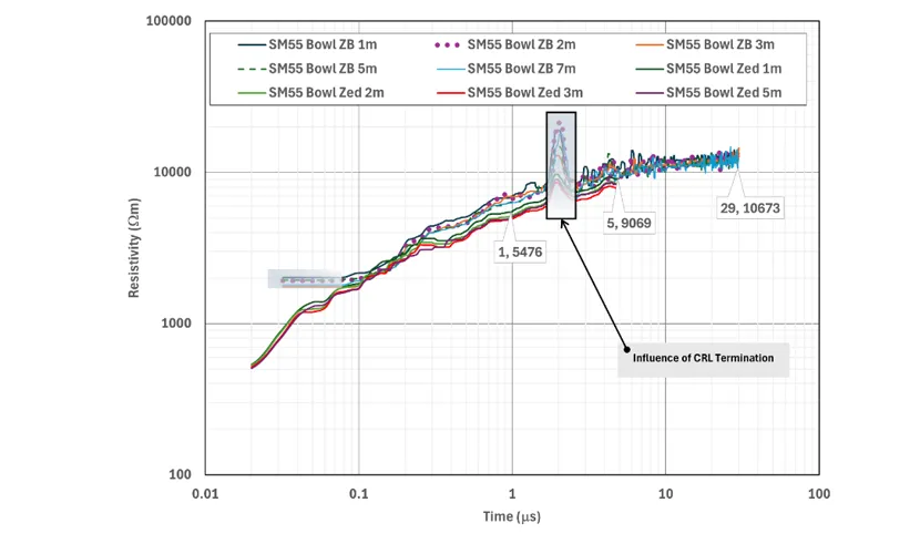
While the reflections from imperfect termination of the CRL in Fig. 25 are small, they upset the measurement of ρ(t) from 1.7 to 3 μs. Tests with both pulse generators show the same, smooth transitions of ρ(t) from 100 ns to 1.5 μs and at 5 μs for all five values of r₂ from 1 to 7 m.

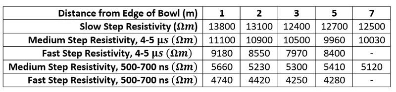
The tendency for increasing ρ(t) in the time range 0.1 … 30 μs in Table 3 matches the corresponding decrease in ρ(f) as from 100 Hz to 1 MHz in [30], developed for locations in Brazil.

Local Footing Resistance & Impedance

Calculations Based on Uniform Soil Model
The Wenner survey results suggest a bottom-layer resistivity of 13,900 Ωm and this was matched by average resistivity of 12,900 Ωm within 7 m of the test hemisphere. With 11 m spacing between adjacent tower legs, the effective perimeter of 44 m gives an estimated R_f = ρ/P = 13,400/44 = 305 Ω.

Measurements with Directional Test Method
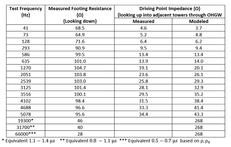
Fig. 26 shows four flexible Rogowski coil current sensors, each wrapped four times around a lattice tower leg. The current from the test source was injected in separate tests, above and below a coil. This was done to measuring the small fraction of current flowing into the tower, and the large fraction upwards into the OHGW and adjacent towers, at test frequencies from 41 Hz to 5078 Hz.

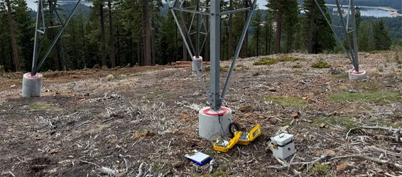
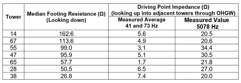
Table 4 shows that the measured footing resistance of the structure increased modestly with frequency, while the impedance looking up increased by a factor of seven. This was the result of the inductive reactance of the OHGW connections to adjacent structures. A spreadsheet model using a chain of series inductance and parallel resistance to ground matched the measured driving point impedance up to 2 kHz. This process was repeated at six other towers, confirming in Table 5 that the multi-grounded OHGW provides a low-impedance path for power frequency fault current.

In all cases, the driving point impedance of parallel structures, connected via the single OHGW, was found to be less than the local structure footing impedance. The measured driving-point impedances in two directions in Table 5 are multiplied by two and plotted against results of a complex impedance calculation for one direction in Fig. 27.

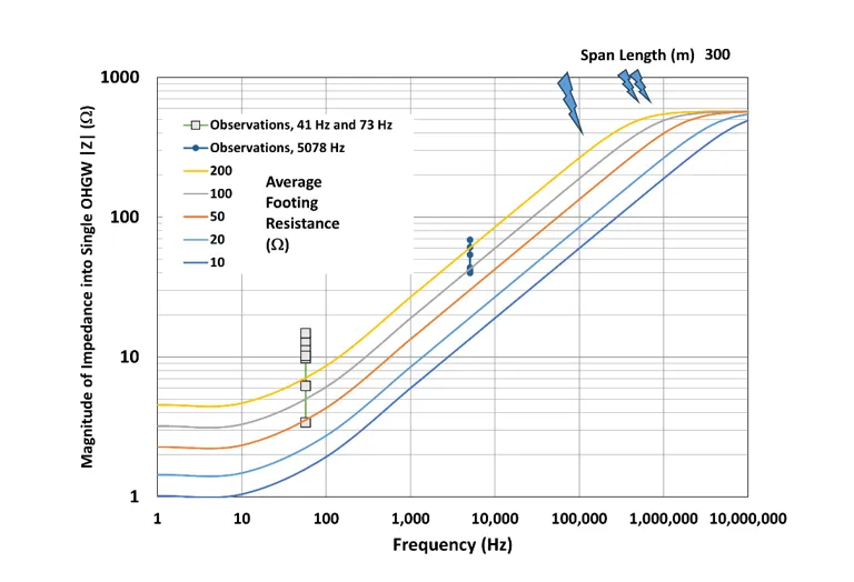
The impedance calculations in Fig. 27 make use of complex numbers in a spreadsheet but they are not complicated. The series resistance per unit length R’ of the single OHGW, the per-unit-length inductance L’ and capacitance C’ and a conductance G’ given by the span length divided by the average footing resistance, are combined using:

In Fig. 27 footing resistance varies as a parameter from 10 ≤R ≤200 Ω, giving 30 ≥G’ ≥1.5 S/m with a 300-m span length typical for this 69-kV line.

The complex reflection coefficient at the far end of the OHGW in Equation 5is typically ρ_L=-1+j0 as the substation ground grid has low resistance compared to OHGW surge impedance Z_gw=√(L’ \/C’ ).

Lightning symbols in Fig. 27 indicate the sine-wave frequencies of 124 kHz for first negative RS, and 516 kHz for subsequent RS. These sine waves have peak current and derivative of (31.1 kA,24.3kA/μs) for the larger, single indicator and (12.3 kA,39.9 kA/μs) for the smaller, double indicator. These frequencies are much higher than those used in the directional tester. Rather than changing the frequency of the test equipment, good results can be obtained in the time domain, by exciting the structure and taking impedance measurements before reflections return from adjacent structures. This is the “Zed Method” described next.

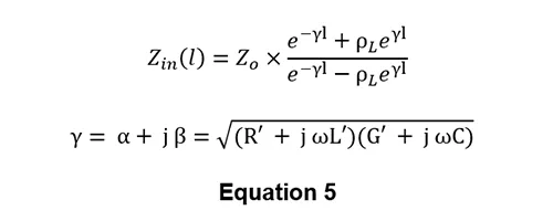
Measurements with Zed Method
It proved to be exceptionally difficult to carry out the Wenner soil resistivity surveys in this work, because the soil was dry and thin and multiple probes were needed to obtain a sufficiently low resistance to permit a nonzero test current. The test time was much faster for the Zed method, which relies on the surge impedance of a wire resting on the ground. Even when the wire is left open, giving ρ_L=+1+j0 in Equation 5, a surge impedance response Z_CRL=√(L’ /C’ ) persists for the two-way travel time along the length of a current reaction lead (CRL). This surge impedance has been found to be 150 Ω≤Z_CRL≤425 Ω in more than 1000 tests. With 200 V excitation, current flow exceeding 0.5 A is achieved, well above the high frequency noise level in field studies.

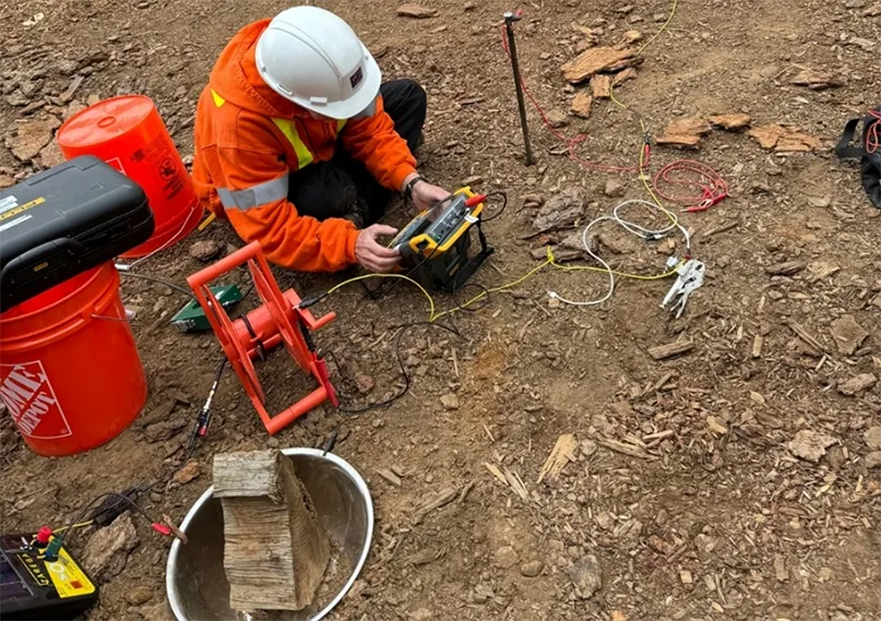
Once the 150-m CRL is laid out along the right-of-way, a computerized instrument with pulse generator, current sensor and digitizers in Fig. 28 is grounded to the structure under test. The active lead from the pulse generator connects to the CRL, and the potential difference from structure to points nearby is measured with a wideband voltage probe with 10 MΩ impedance. This is large enough that there is minimum loading when a second wire over ground, the “Remote Potential Lead”, is used to minimize coupling to any buried counterpoise.

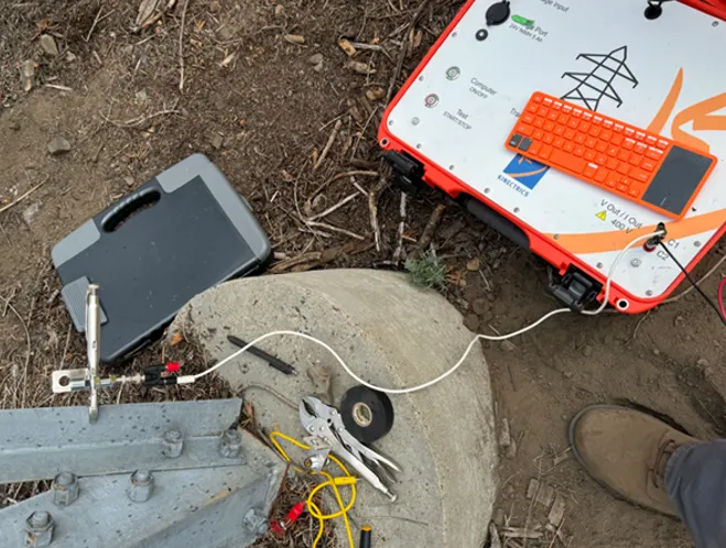
In these tests, the CRL was terminated in a hemisphere such as in Fig. 29 to save some time. Typically, the hemisphere impedance (Table 3) was much greater than the surge impedance of the CRL.

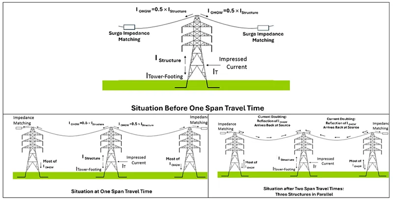
Fig. 30 illustrates the need to carry out a measurement in a time window. The voltage rise at tower base stabilizes as the I_OHGW flows in two directions away from tower top. The “Surge Impedance Matching” is not a physical resistor – it is just the continuation of the wire itself over ground, just like the CRL surge impedance. After one span travel time, about 1 μs for a 300-m span length at the speed of light, these small portions of the impressed current arrive at the adjacent two structures. After two span travel times, “knowledge” that there are structures nearby arrives back at the structure under test.

The purpose of the CRL is to provide a stable surge impedance path for the impressed current for the two-way travel time, at most 2 μs, to establish Z_f of a single tower.

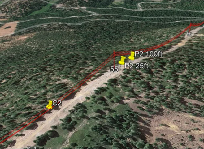
The sketch in Fig. 31 shows the arrangement of test leads. Transient potentials were measured with a high-impedance probe, grounded to structure 55 and with the live lead connected to ground rods at distances of 25’ (7.6 m) and 100’ (30.5 m) from the leg receiving the impressed current. The difference in transient potential between the two points is used to estimate transient resistivity ρ(t) as well as to correct the readings to infinite distance.

Comparison of Results
With this comprehensive test program, it was possible to compare:

• Soil resistivity using the bowl test versus results from interpretation of Wenner surveys
• Soil resistivity using the bowl test, comparing results at low frequency with ρ(t) in selected time intervals from 500 to 1400 ns, used in the Zed method analysis
• Transient soil resistivity at the structure versus low-frequency resistivity
• Structure impedance with directional test (41 – 5078 Hz) compared to transient impedance

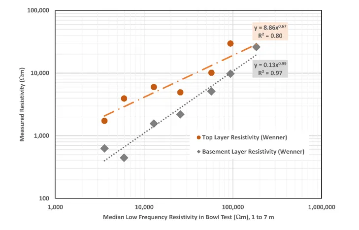
The Wenner survey results suggested a complicated three- or four-layer soil model that was different at every structure. Fig. 32 shows a strong relation between the resistivity values from the bowl test and the resistivity value fitted to the bottom (basement) layer. The values for the hemisphere test on the horizontal axis are the median of results at distances from 1 to 7 m, using the DC excitation in Fig. 21.

The Wenner survey results suggested a complicated three- or four-layer soil model that was different at every structure. Fig. 32 shows a strong relation between the resistivity values from the bowl test and the resistivity value fitted to the bottom (basement) layer. The values for the hemisphere test on the horizontal axis are the median of results at distances from 1 to 7 m, using the DC excitation in Fig. 21.

The comparison of transient resistivity in Fig. 33 with the same horizontal axis as Fig. 32 makes use of the readings taken 1 m from the edge of the bowl, to make them comparable to readings taken in past research. However, these tests did not find much difference in the resistivity estimates taken anywhere from 1 to 7 m from the bowl, suggesting that the uniform soil model is reasonable for these dimensions.

The final comparison reported here is the measured structure impedance at three selected times, compared to the low-frequency resistance reported in the directional tests. Fig. 34 shows that the 5078-Hz values in the directional test have a nearly linear relation to the 41-Hz values with power-law exponent of 0.82, and Pearson regression coefficient of R2 = 0.87.

The impedance values for each structure varied with time, with lower values in the period 500-700 ns, rising a bit for median values of Z(t) for 800 ≤t ≤1100 ns and, following the curve of ρ(t) in Fig. 25, rising further for 1100 ≤t ≤1400 ns. The fitted power-law exponents decrease from 0.82 to the 41-Hz values to 0.56 for 800 ≤t ≤1100 ns , 0.52 for 800 ≤t ≤1100 ns and 0.32 for 500 ≤t ≤700 ns. These trends have been reported previously based on test results from structures that were insulated from their OHGW, prior to successful development of directional test equipment.

Conclusions

Despite a wide range of global lightning ground flash density Ng, the lightning performance of a transmission line is expected to fall in a narrow security range, from Class C (<4 outages per 100 km per yr) of 69 kV lines up to Class A (< 0.5 outages per 100 km per yr) for UHV lines.

The shielded 60-69 kV transmission lines with a decade of service in 1955 offered reasonably good reliability, usually achieving at least Class C. Some of these lines achieved better security levels after rebuilding to improve shielding, reduce footing resistance and increase the surge impedance coupling coefficients. These lines are some of today’s candidates for rebuilding projects as placeholders on valuable urban right-of-way.

Improved understanding of counterpoise for grounding leads to advice not to exceed its effective length, given by square root of resistivity (Ωm) and ramp rise time of 2 μs. Thus, l_eff in 200 Ωm soil is 20 m, and l_eff in 10,000 Ωm soil is 141 m. Since there is a large tower-to-tower variation in resistivity, each earthing treatment needs to be customized. This added test burden ensures that programs for improved earthing are not as effective as fitting of TLSA, UBGW and/or CICA in line rebuilding projects to improve or restore lightning performance to the desired security class.

Some of the testing burden can be used by making transient resistivity tests with a single, buried hemisphere rather than traditional vertical probes at multiple locations in Wenner or Schlumberger tests. The bowl tests are much more efficient in high-resistivity soil where it is difficult to establish probe resistance. The results are not sensitive to the test equipment and show a smooth transition in ρ(t) in the time range from 100 ns to 1 s, allowing for some disturbance from travelling wave effects in the connection to remote electrode.

Acknowledgements
Development of the Zed method, including commercialization of the Zed Meter®, was supported by EPRI, EDM and participating electrical utilities in the USA, Canada and around the world. Kinectrics supported the participation of the authors in revision of IEEE Standard 81-2025.

References

[1] EPRI, EPRI AC Transmission Line Reference Book – 200 kV and Above, Third Edition (the Red Book), Palo Alto, CA: EPRI 1011974, December 2005.
[2] ESKOM, The planning, design and construction of overhead power lines, Johannesburg: Crown Publications cc, May 2010.
[3] CIGRE Study Committee B2: Overhead Lines, Overhead Lines, Cham, Switzerland: Springer Nature, 2017.
[4] CEATI International, “Best Practices Guide for Extra High Voltage (EHV) AC Overhead Transmission Line Design – Electrical Aspects,” CEATI Report T163700-3398A, Montreal, Canada, February 2019.
[5] K. Hamachi_LaCommare and J. Eto, “Cost of Power Interruptions to Electricity Consumers in the US,” Berkley National Lab LBNL-58164, Berkley, CA, February 2006.
[6] K. Hamachi LaCommare and J. H. Eto, “Understanding the Cost of Power Interruptions to US Electricity Consumers, LBNL-55718,” Ernst Orlando Lawrence Berkeley National Laboratory, Berkley, CA, September 2004.
[7] IEEE, IEEE Guide for Improving the Lightning Performance of Transmission Lines, Piscataway, NJ: IEEE Standard 1243-1997, Reaffirmed 2008, September 2008.
[8] IEEE Power & Energy Society, Transmission and Distribution Committee, IEEE Standard 1410-2010: IEEE Guide for Improving the Lightning Performance of Electric Power Overhead Distribution Lines, New York: IEEE Standards Association, 2011 Jan 28.
[9] CIGRE WG 33.01, Guide to Procedures for Estimating the Lightning Performance of Transmission Lines, Paris: CIGRE Technical Brochure 63, October1991 revised 2021.
[10] CIGRE WG C4.23, “Procedures for Estimating the Lightning Performance of Transmission Lines – New Aspects,” CIGRE Technical Brochure 839, Paris, June 2021.
[11] IEEE-SA Board of Governors and IEEE Power and Energy Society, IEEE Recommended Practice for Overvoltage and Insulation Coordination of Transmission Systems at 1000 kV AC and Above, New York, NY : IEEE Standard 1862-2014, 15 May 2014.
[12] T. Miki, M. Miki, S. Watanabe and R. Yamada, “Applying EGLAs on Transmission Lines in Japan: Overview of Experience & Lightning Outage Data,” in 2023 INMR World Congress, Bangkok, 2023.
[13] Ohio Brass Company, Lightning Performance of Typical Transmission Lines, Second Edition, Mansfield, OH: Ohio Brass Company Publication 1321-H, 1955.
[14] CIGRE WG 33.01, Guide to Procedures for Estimating the Lightning Performance of Transmission Lines, Paris: CIGRE Technical Brochure 63, 1991.
[15] EPRI, Transmission Line Reference Book: 115-345 kV Compact Line Design, Palo Alto, CA: EPRI 1016823, 2008.
[16] W. A. Chisholm, “Arrester Protection of Lower Voltage Circuits on Multi-Voltage Towers: Issues & Opportunities,” in 2019 INMR World Congress, Tucson, AZ, October 20-23, 2019.
[17] W. A. Chisholm, “Balancing the Budget for Renovating Lines: Groundwires, OPGW, Insulation, Earthing & Arresters,” in INMR 2023 World Congress, Bangkok, Thailand, 14 November 2023.
[18] CIGRE Working Group B2.21, “On the use of Power Arc Protection Devices for Composite Insulators on Transmission Lines,” CIGRE Technical Brochure 365, Paris, December 2008.
[19] CIGRE WG C4.39, “Effectiveness of line surge arresters for lightning protection of overhead transmission lines,” CIGRE Technical Brochure 855, Paris, December 2021.
[20] CIGRE WG C4.407, Lightning Parameters for Engineering Applications, Paris: CIGRE Technical Brochure 549, August 2013.
[21] EPRI, Transmission Line Reference Book, 345 kV and Above, Second Edition, Palo Alto, CA: EPRI, 1982.
[22] J. Takami and S. Okabe, “Observational Results of Lightning Current on Transmission Towers,” IEEE Transactions on Power Delivery, vol. 22, no. 1, pp. 547-556, January 2007.
[23] W. A. Chisholm and S. de Almeida de Graaff, “Adapting the Statistics of Soil Properties into Existing and Future Lightning Protection Standards and Guides,” in 2015 International Symposium on Lightning Protection (XIII SIPDA), Balneario Camboriu, Brazil, 28 September – 2 October 2015.
[24] J. Clayton and F. Young, “Estimating Lightning Performance of Transmission Lines,” IEEE Transactions on Power Apparatus and Systems, vol. 83, no. 11, pp. 1102-1110, November 1964.
[25] M. Darveniza, F. Poplansky and E. Whitehead, “Lightning Protection of EHV Transmission Lines,” Electra, vol. 041, no. 2, pp. 39-69, 1975.
[26] E. Koncel, “Potential of a Transmission-Line Tower Top when Struck by Lightning,” Transactions of the AIEE Part III, vol. 75, no. 3, pp. 457-462, January 1956.
[27] T. Udo, “Estimation of Lightning Current Wave Front Duration by the Lightning Performance of Japanese EHV Transmission Lines,” IEEE Transactions on Power Delivery, vol. 8, no. 2, pp. 660-668, April 1993.
[28] F. Silveira and S. Visacro, “Lightning Performance of Transmission Lines: Impact of Current Waveform and Front-Time on Backflashover Occurrence,” IEEE Transactions on Power Delivery, vol. 34, no. 6, pp. 2145-2151, December 2019.
[29] F. Silveira, L. Pires, Y. C. Costa and S. Visacro, “A discussion on approaches to consider current front time of linearly rising waveforms applied to the assessment of the lightning performance of TLs according with typical range of backflashover critical currents,” Electric Power Systems Research, vol. 245, p. 111630, August 2025.
[30] CIGRE WG C4.33, Impact of soil-parameter frequency dependence on the response of grounding electrodes and on the lightning performance of electrical systems, Paris: CIGRE Technical Brochure 781, October 2019.
[31] CIGRE WG B2.56, Ground Potential Rise at Overhead AC Transmission Line Structures during Power Frequency Faults, Paris: CIGRE Technical Brochure 694, 2017 07.
[32] L. Grcev, B. Markovsi and M. Todorovski, “Lightning Efficient Counterpoise Configurations for Transmission Line Grounding,” IEEE Transactions on Power Delivery, vol. 38, no. 2, pp. 877-888, April 2023.
[33] W. A. Chisholm, “Evaluation of Simple Models for the Resistance of Solid and Wire-Frame Electrodes,” IEEE Transactions on Industry Applications, vol. 51, no. 6, pp. 5123-5129, November/December 2015.
[34] M. Mokhhtari, A. de_Araujo, D. Clark, S. Robson, M. Albano, M. Hadad, M. Shaban and D. Guo, “An Analytical Model for the Low Frequency Earthing System of the T-Pylon Transmission Tower,” in 59th International Universities Power Engineering Conference, Cardiff, UK, September 2024.
[35] IEEE Power and Energy Society, IEEE P81/D4 – Approved Draft Guide for Measuring Earth Resistivity, Ground Impedance, and Earth Surface Potentials of a Grounding System, New York, NY: IEEE, D4 Update January 2025, Approved 2025-06-19.
[36] W. A. Chisholm, E. Petrache and C. L. Mauff, “Field Tests of Square and Double Exponential Pulses for Transient Resistivity Measurements using Wenner Arrays and Hemispheres,” Electric Power Systems Research, vol. 233, no. 110499, p. 9pp, 28 May 0224.
[37] S. Visacro, F. Silveira and C. Oliveira, “Measurements for Qualifying the Lightning Response of Tower-Footing Electrods of Transmission Lines,” IEEEE Transactions on Electromagnetic Compatibility, vol. 61, no. 3, pp. 719-726, June 2019.