Most transmission applications require verifying electric fields that, if exceeding certain thresholds, can cause corona discharges, dielectric breakdown and electromagnetic interference. Since insulators are associated with complex conducting structures, estimating electric field strength at selected points along strings, corona rings and their immediate surroundings requires simulating the complete tower along with conductors. This edited contribution to INMR by experts at INTEGRATED Engineering Software in Canada illustrates how such modeling has been applied to a 3-phase, 115 kV transmission tower using COULOMB, a 3D electrostatic field solver.
Model Geometry
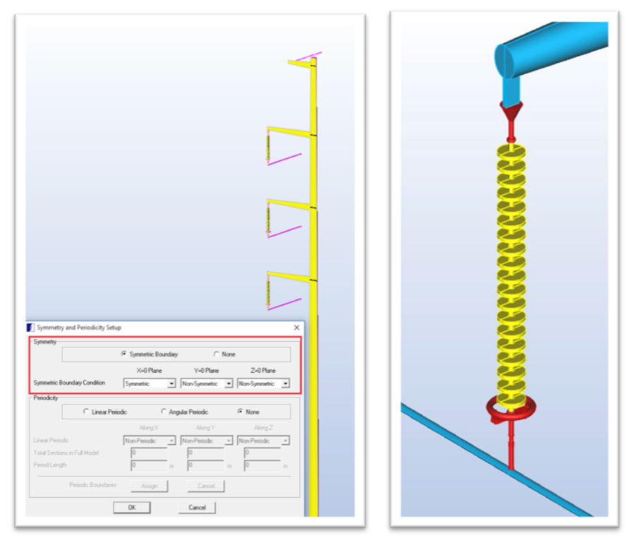
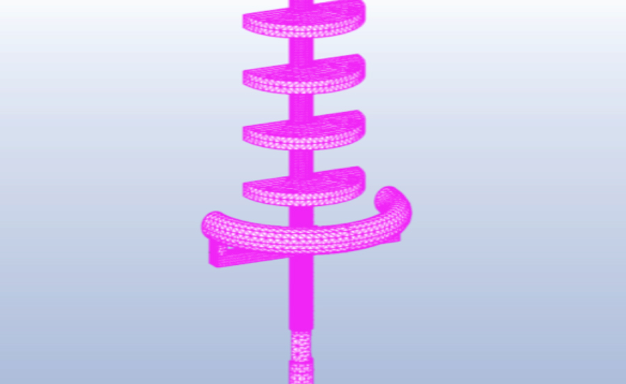
Fig. 1a depicts a transmission tower, imported from a STEP file, which is about 30 m high and supports Phases A, B and C as well as the ground wire. Conductors are about one inch (2.5 mm) diameter and ground wire about half-inch diameter and these are modeled to a length of about 5 m. Fig. 1b shows the conductor attached to the suspension insulator and its corona ring. The whole model is symmetric about the X = 0 plane. Figs. 2a and 2b show the symmetry set-up and non-symmetric model respectively. The symmetric model is used in this example.
Materials & Boundary Conditions
The tower and conductors are made of aluminum and the ground wire is steel (linear). The insulator type used here has silicone rubber sheds bonded onto a glass fiber filled (FRP) rod. The corona ring and fixture are made of copper. Dielectric constants for all these materials are calculated at a power frequency of 60 Hz. Ground wire and tower are at 0 V while conductors, along with their corona ring structures, are assigned 115 kV at phase angles of 0º, 120º and -120º from the top.
Meshing
Since this model involves a wide-open space around the device, problems involving such open regions are best handled by the Boundary Element Method (BEM), where only the ‘active’ regions require discretization. Fields can be calculated anywhere in 3D space and this allows modeling true geometric curvature rather than only straight-line approximations. Models with thin layers and extreme aspect ratios are handled more easily.
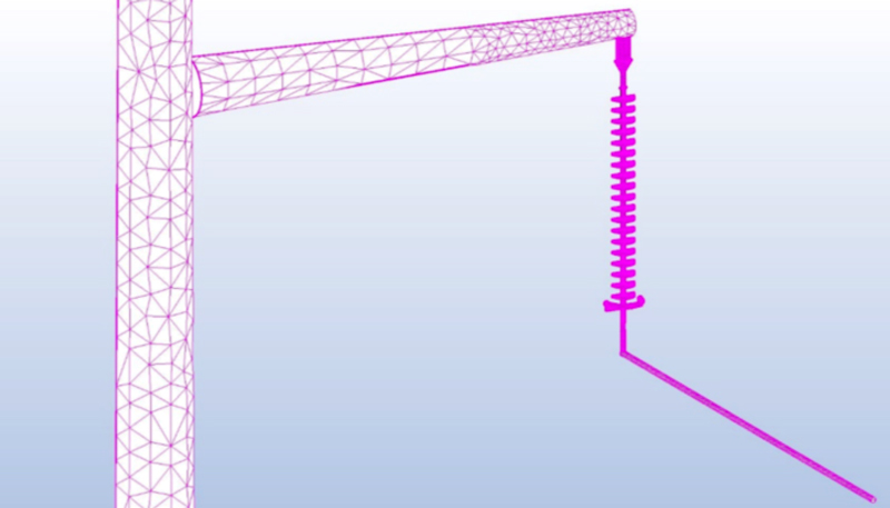
Using BEM formulation, equivalent charges that support the specified boundary conditions are determined. From these, equivalent charges, electric potential and electric field are calculated by appropriate integration, effectively smoothing out the discretization error. BEM is more accurate and faster than FEM-based formulation. Figs. 3a and 3b depict global and local views of the 2D triangular mesh.
Since all materials are linear, the BEM solver needs to solve for unknowns only at the boundaries and requires only a 2D triangular mesh on all surfaces. Elements can be assigned automatically throughout the model and local mesh density can be refined manually when accurate results are required.

This model contains about 101,000 2D triangular elements and requires an optimal RAM of about 14 GB. Without symmetric conditions, the model would require about 183,000 2D elements and a RAM of about 48 GB, i.e. a 4-fold increase in memory requirement and a significant increase in computation time. Symmetry about any principal plane should therefore be used to allow faster simulation.
Physics & Solver Settings
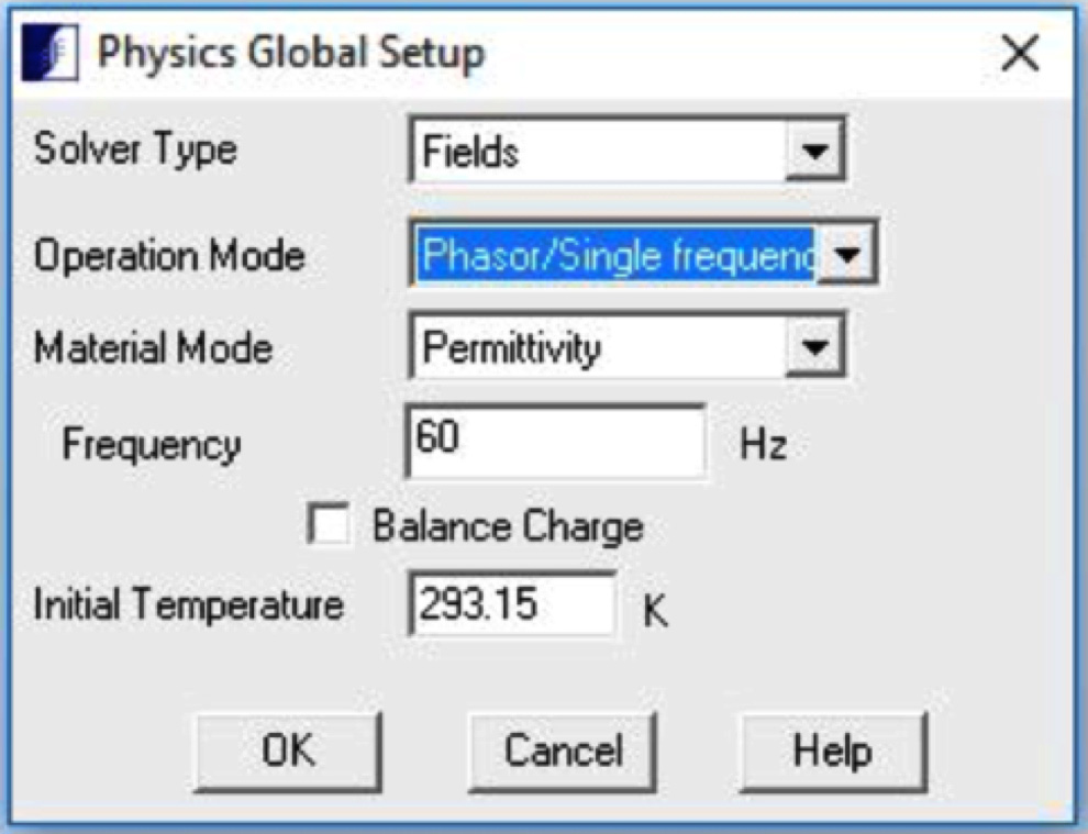
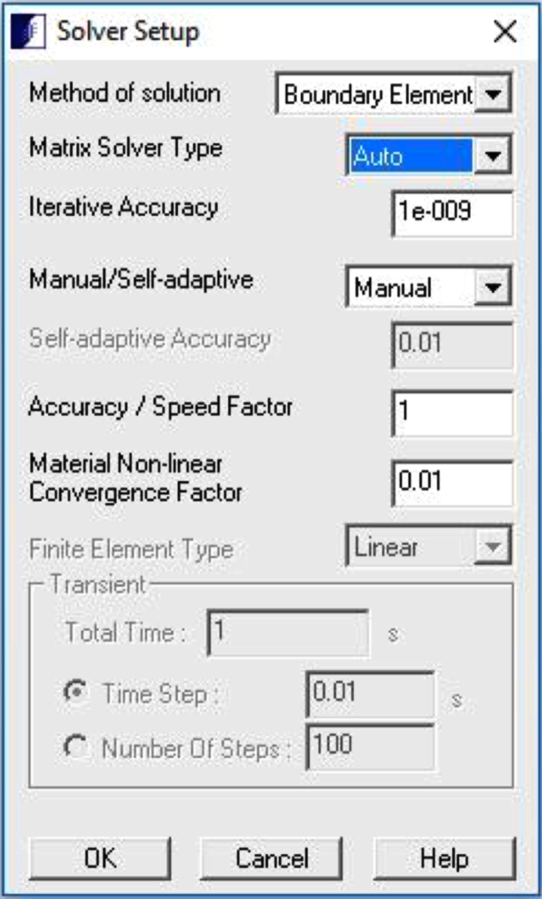
Fig. 4a shows the physics settings. The solver type is set to ‘Fields’. The operation is at a single frequency of 60 Hz. Charge balance is turned off. In balanced mode, the solver will force the total charge in the model to add to zero. In this mode, there is need for a reference potential to be set somewhere. In the unbalanced mode, the surroundings around the model will hold whatever excess charge is required and the potential at infinity will be zero, requiring no potential reference. Only ungrounded sources, such as a battery, require charge to be balanced in the model.
Fig. 4b provides the solver settings. In the solver set-up, BEM is the method of solution. The matrix solver type can be set to ‘Direct’, ‘Iterative’ or ‘Auto’. In auto mode, COULOMB automatically determines the best solver without need for user interaction. The direct solver is robust but requires more time than the iterative solver. Meshing can be manual or self-adaptive. In this particular case, the model was meshed manually for better local results.

Post-Processing & Results
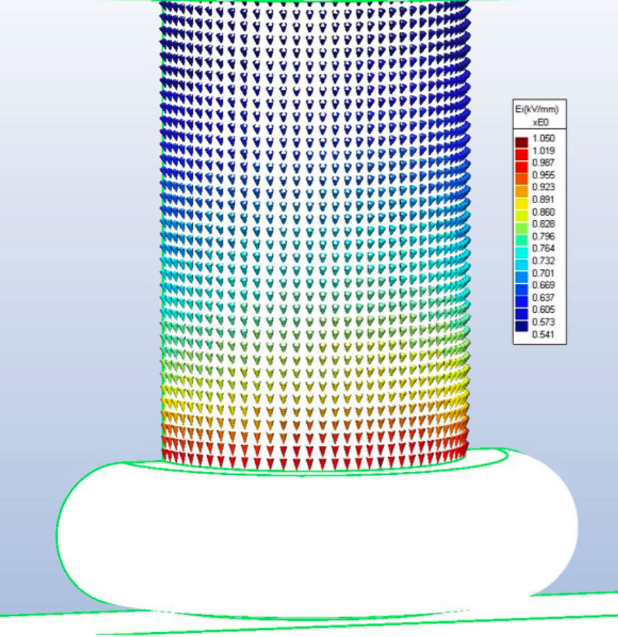
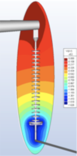
As can be seen, the corona ring reduces the electric potential gradient and lowers maximum electric field value below the corona inception threshold. Figs. 5a and 5b show a comparison of the electric field near the bottom of an insulator, with and without corona ring. This total field at time angle 0º is directed downwards. As can be observed, maximum field has been reduced from about 1.05 kV/mm to 0.41 kV/mm using the corona ring.
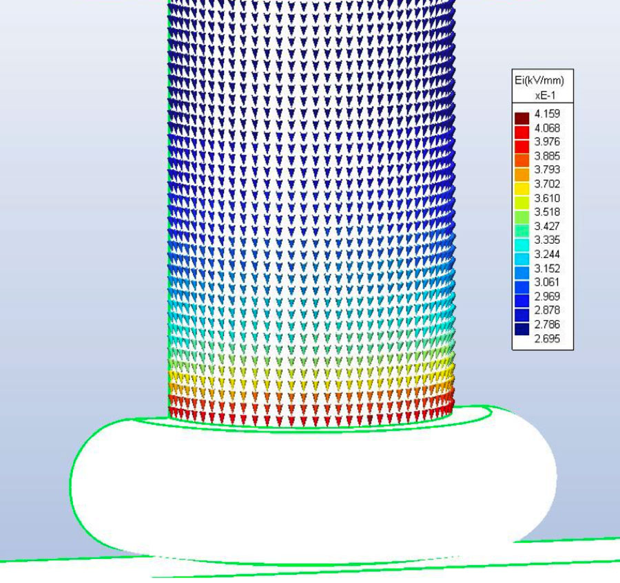

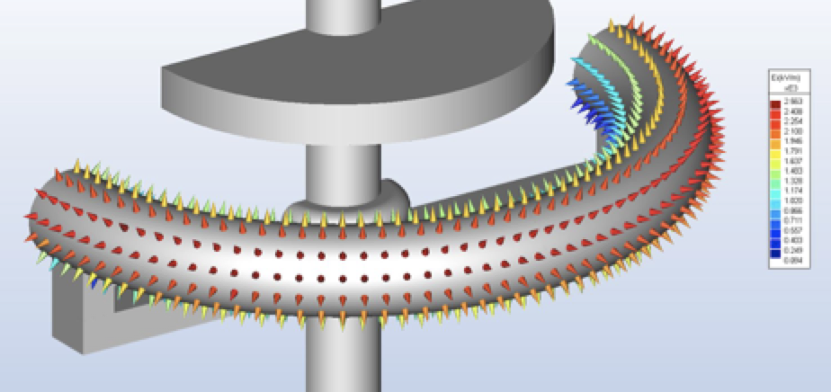
Fig. 6 shows an arrow plot of the electric field on the corona ring.
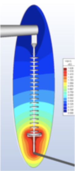
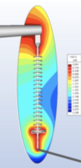
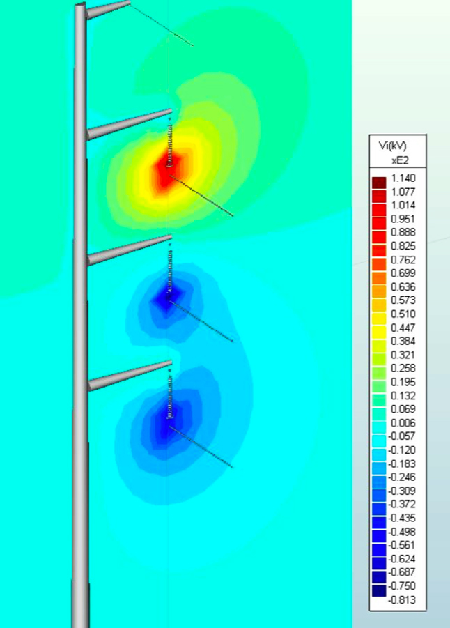
Figs. 7a, 7b, and 7c plot the potential contours on a plane through the mid-section of the top insulator at time angles 0º, 90º and 180º. Initially, the maximum potential near the conductor equals the peak value of line voltage as a cosine function, which is the square root of 2 times 115 kV i.e. 162.6 kV. At 90º, the maximum potential is 0 kV and at 180º it is -162.6 kV. Fig. 8 shows the potential contours of all three conductors on the X = 0 plane.
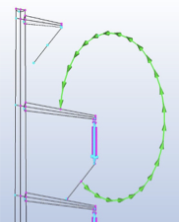
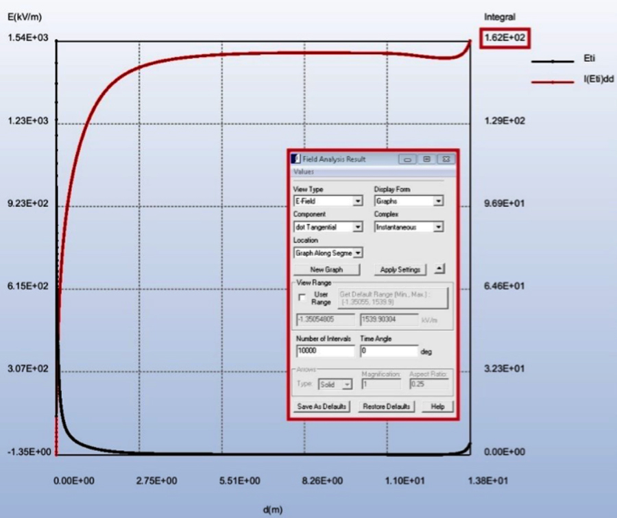
To verify the simulation, tangential electric field between points a and b can be plotted and its line integral calculated, which must equal the potential difference between the two points.
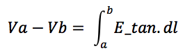
Fig. 9a shows an arc drawn from a point on the top conductor to a point on the tower. In Fig. 9b, a graph of tangential electric field is plotted and integrated along this segment. This integral equals 162 kV, which is the potential difference between the two points at time angle 0º.
The value of electric field surrounding a line must be lower than some maximum allowable limit for the safety of personnel and the public. COULOMB can efficiently simulate these requirements. For magnetic fields, the same model can be simulated using the 3D magnetostatic field solver, AMPERES. In this case, the excitation has to be the RMS value of current flowing through the conductors.