This edited contribution to INMR by Rene Hummel (Germany) and Mark Fenger (Canada) of Kinectrics describes the commissioning test of 3-phase 400 kV XLPE cable systems using on-site Partial Discharge (PD) testing. Each cable system in this case is more than 22 km in length and consists of 33 cross-linked joints as well as 6 end terminations.

To perform the test, the cable system was energized with a resonant test set to 330 kV for a period of 60 minutes. Three teams of technicians simultaneously measured PD at different cable joints using high-frequency current transformers (HFCTs) and mobile PD test equipment in a process referred to as ‘joint-hopping’.

Selection of appropriate measurement frequencies and verification of sufficient sensitivity are discussed and results analyzed.

---

High voltage (HV) cable systems are the backbone of energy networks around the globe. While their purchase is costly, the installation and required civil works can be even more expensive. Full turnkey projects for long lengths of HV or EHV cable, installation, civil works, substations and associated needed infrastructure can exceed $1 billion. Once installed and energized, HV and EHV transmission class cables are typically critical assets for the energy grid and must not fail in service. To assure proper production, installation and life cycle management of such assets, the IEC, IEEE and CIGRE have all issued multiple Guides, suggestions and standards – all requiring proper testing of HV cables.

Before HV & EHV cables and cable components leave the factory, they must undergo a series of tests to ensure that they meet contractual specifications, which are often based on the aforementioned standards and guides. Some tests are designed to check the mechanical integrity of the cable conductor, the dimensions and multiple parts of the extrusion process during manufacturing.
To test the insulation of the cable, HV testing with voltages exceeding rated operating voltage (U0) combined with Partial Discharge (PD) measurement are widely used. These tests shall assure that no life limiting production-related damage or impurities are present in the insulation of the cable system.

Successful testing in the factory requires trained personnel and adherence to cable factory testing standards. Ideally, these tests are carried out in a controlled environment such as shielded rooms to reduce external background noise. However, even the most rigorous factory testing cannot guarantee that the cables will be installed correctly or that they will not be damaged during transport or laying.

Once cables are delivered to site and installed, most future owners require commission tests before accepting ownership. Such tests are designed to detect possible damage that might have been inflicted during transport or laying. Special focus lies on the accessories, which are often installed in the field under conditions that are far from the clean, shielded room conditions of factory setups. In fact, the primary purpose of on-site testing is to detect possible issues in the cable system resulting in limiting life.

According to CIGRE studies based on a population of 26,494 km of HV and EHV cable tested with AC (20 Hz – 300 Hz), only 0.01% of the cables systems showed non-passing issues in the cable sections themselves. However, the non-pass rates for terminations and joints were 2.8% and 0.75% respectively.

For on-site testing, overvoltage tests above nominal voltage phase-to-ground (U0) and in combination with PD testing is now state-of-the-art. IEC and CIGRE both state requirements in regard to voltage levels and setup of PD measurement equipment. These requirements are rigorous to assure proper testing of HV cable systems to avoid both false positive and false negative test outcomes. Often, the parties carrying out the on-site tests follow such requirements, particularly in regard voltage levels and test durations.

To energize HV and EHV cables, especially with elevated voltages, huge and expensive generator-transformer test sets would be needed. Their size and weight would put many challenges in the project management involved in the testing. Therefore, to reduce the size and weight of the voltage sources for such a commissioning test, mobile, modular Resonant Test Systems (RTS) are often used to energize the cables. Many HV RTS usually have a fixed inductance. Together with the capacitance of the cable system, a resonance circuit is established and by means of tuning the frequency, the resonance frequency between 20Hz and 300Hz is being established as per Clause 16.3 of IEC 60840 and IEC 62067.

The longer the cable system at a certain voltage class, the greater the capacitance and resistive losses in the cable system under test. For long cable systems, such as the 22 km cable system described here, multiple RTS need to be used in series and parallel to drive the needed current and therefore voltage for the overvoltage tests.

IEC and CIGRE state clear requirements concerning the PD measurement, required sensitivity, maximum allowable PD from a cable system and thus the maximum background noise. These requirements are justified and are important to achieve. Unfortunately, for long cable systems, these requirements are seldom met, especially the demands for background noise. Even with state-of-the-art PD test systems, obtaining a background noise of less than 5pC can be challenging to impossible, based on the surroundings of the test area. For the time being, the only way to conduct PD measurements is by trying to reduce background noise and varying the PD measurement frequencies (center frequency) by assuring proper sensitivity at the same time.

Challenges of PD Measurement for Long HV Cable Systems

The primary challenge of PD measurement for long HV cable systems is the high attenuation of the PD signals and, as well, further magnitude deterioration at accessory/cable interfaces. This attenuation is caused by the resistance, inductance and especially capacitance of the cable and increases with cable length. As a result, the PD signals that reach the PD measurement sensors are weaker than for a shorter cable. This can make it difficult to detect and measure PD signals, especially at low levels. Even low levels of PD can indicate issues within the cable insulation and can lead to severe and even catastrophic failures with danger to assets and safety.

Another challenge is the potential for interference from external sources. In general, the cable acts like an antenna for airborne noise. The longer the cable, the better the antenna function. Interference can come from a variety of sources including power lines, other electrical equipment regulated by power electronics such as rotating machines, wireless networks, and even the grounding network. It can be especially important to filter out interference when possible PD signals are weak.

Test Setup

Cable System
The cable under test is specified as a 230 kV / 400 kV cable with U0 = 220 kV and Umax = 420 kV with a length of 22 km and a copper conductor with a minimum diameter of 2500 mm². Each phase of the 3-phase cable is sectionalized by 33 joints thus creating 34 cable sections. Open-air end terminations are installed at one end of the cable. On the other GIS end terminations are present. The end terminations at both sides are grounded directly.

What Cable End to Energize From?
Connecting an external voltage source such as an RTS to a GIS is possible by means of special adapters that require trained personnel to be connected correctly and must also be handled with care. Moreover, they have an economic impact on testing costs. While these costs are small in relation to the total project cost of the cable installation, they can become a significant factor in relation to the cost of commissioning testing by itself.

Testing through the GIS would result in the energization of more parts of the GIS system than the cable terminations only. These additional parts often have current transformers (CTs) or voltage transformers (VTs) installed that have stricter limitations concerning possible overvoltage and testing voltage frequencies. Depending on manufacturer of the GIS and CTs and VTs, the testing voltage frequencies are usually limited to 50 Hz to 80 Hz. This is a significant difference to the aforementioned 20 Hz and 300 Hz (IEC 60840 and IEC 62067) for cable testing.

These limitations would increase number of RTS systems needed since more power would be necessary to bring the resonant frequency up to 50 Hz – 80 Hz rather than slightly above 20 Hz. This increases complexity of the HV voltage source setup and therefore testing costs. Thus, it was decided to energize the cable from the open air end termination side.

Joints
In each phase, 33 joints connect the 34 sections of the cable to each other.

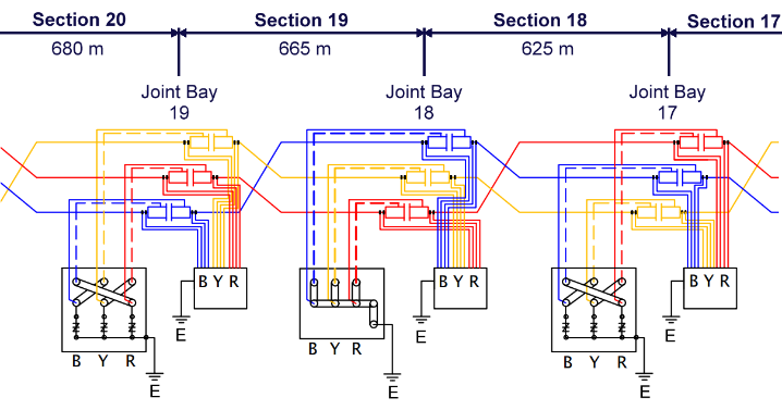
The individual cable sections between the joints vary from 610 m to 700 m. At every third joint bay, the cable sheaths are grounded. For the other joint bays, cross bonding is installed with over-voltage arresters towards ground.

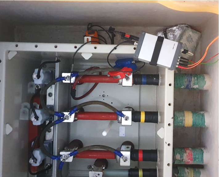
Measurement Setup
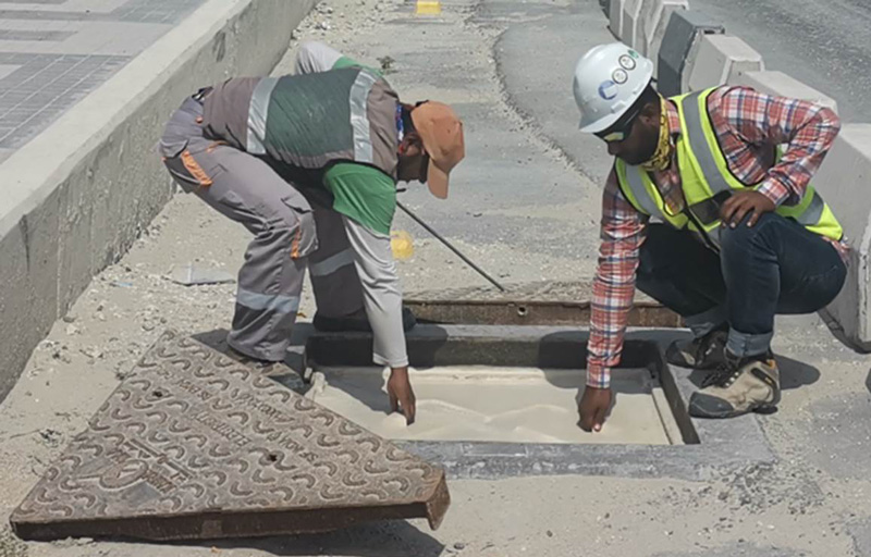
Long AC high-voltage (HV) cables are installed with cross-bonding joints to reduce circulating currents in the cable screens. During AC commissioning testing of each phase individually, the cross-bonding configuration of the cable screens must be inactive and a straight-through cable screen configuration must be established. These configurations are often done in link boxes, which can be accessed from above. Sometimes these link boxes are above ground, but are often located in manholes or just below the surface in joint bays, referred to as ‘coffin boxes’.

HFCT
Link boxes provide easy access to the screens of the joints and often allow for the easy installation of High Frequency Current Transformers (HFCTs). HFCTs are non-invasive sensors that can be clamped around the cable screens to detect PD signals. The main advantage of placing HFCTs in link boxes is their proximity to the joints. This allows for the detection of PD signals with high sensitivity and accuracy.

In a factory environment, where individual cable reels and accessory components are tested, coupling capacitors are typically used to measure PD signals, as stated in the IEC 60270. This is so because the test objects in a factory environment, largely, behave like lumped capacitances. Coupling capacitors are connected in parallel with the cable conductor and provide a path for the PD signals to flow to the measuring equipment. However, coupling capacitors are not feasible for long cable systems since (1) these constitute distributed impedances and (2) are subject to attenuation of high frequency signals such as PD.

Cigre B1.28 states: “For shorter lengths of cable systems, terminal PD measurements can be performed, whereas for longer lengths of jointed cable systems a distributed PD measurement should be performed.” [1] This means that for long cable systems, it is important to measure PD signals at multiple locations (joints) along the cable length.

HFCTs are often the best sensors for distributed PD measurement because they are non-invasive and can be installed at any location along the cable route without the need to include PD sensors in the joints themselves.

Center Frequencies Setup
Many PD measurement systems allow the operator to determine the center frequency for each sensor. The main goal of such setting is to ensure proper PD signal reception and the proof thereof. To reduce the background noise, changing the center frequency can be helpful too, as long as it can be assured that PD signals are not missed.

The ultimate goal is to a good signal to noise ratio (SNR), with a high decoupling of possible PD signals and low background noise. Unfortunately, the background noise can be different at every joint position.

The center frequencies for the PD measurement should be chosen with care based on the setup and used sensors. Some users have the tendency to view the manufacturers transfer function of a given sensor and assume this will be the frequency response of the total measurement system. Sometimes they even perform what many people call “calibration” before arriving on site.

Using a calibrator to inject a signal into the HFCT is a sensitivity check, but should not be mistaken with a calibration according to the IEC standards for factory measurements on cable components or short cable lengths. For this case it must be noted, that for long lengths of cables, the cable system does no longer act like a lumped capacitance and the assumptions in IEC 60270 is no longer meaningful.

A sensitivity check of the HFCT will give the scale factor that can be used to convert the output of the HFCT to the actual PD magnitude. This scale factor is described as k in the IEC 60270. This scale factor is valid for the selected testing center frequency and bandwidth. It will most likely stay within +/- 5% for another HFCT of the same model.

In Fig. 4, the blue line represents an almost ideal transfer function of an HFCT. Operating the HFCT in the frequency range where the blue line is horizontal would be optimal, as the scale factor of the HFCT would the constant – at least in theory.

With the green line representing the FFT of the noise, the difference between the blue and the green line would be the Signal-to-Noise Ratio (SNR). Clearly, the higher the frequency, the higher the SNR. This can be illustrated in the following real background noise measurement at site.

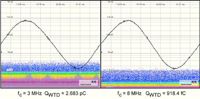
Fig. 5 shows the background noise at 2 different center frequencies using the same scale factor (around k =5). Sometimes this leads to the misconception that the center frequency should be very high to obtain a good SNR or even that the center frequency can be chosen at will as a low background noise is supposedly the most admirable goal during test. Sometimes there is the attempt to change the center frequency at every joint to obtain the lowest background noise. Such procedure neglects the fact, that the HFCTs, the cable leads from the joint to the link boxes and the cable system itself, just to name the most important ones, create a complex network of impedances.

Such complex network will result in a frequency response that does not resemble the blue line in Fig. 4. The effective frequency response can show multiple resonance frequencies that affect sensitivity of the PD measurement at different center frequencies. When viewed in the frequency spectrum, there will be frequencies with high attenuation and frequencies with high amplification.

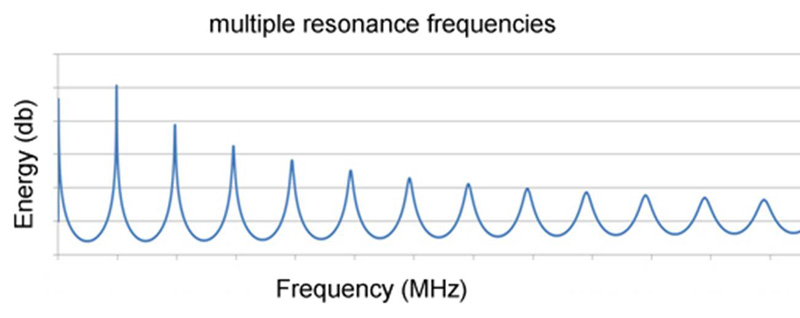
Fig. 6 shows an exaggerated plotted example of multiple resonance frequencies. It shows multiple areas of amplification and attenuation combined with attenuation towards higher frequencies. The attenuation towards higher frequencies is symbolic of the attenuation of signals along the cable.

If the measuring center frequency is set to a position where there is a lot of attenuation/damping visible in the spectrum, the background noise may appear to be low. Inexperienced persons might conclude that this frequency is ideal for getting close to the desired background noise level of less than 5 pC, as suggested in IEC and CIGRE. This is sometimes emphasized by the fact that the scale factor k of the HFCT at this frequency is similar to other center frequencies that are +/- 1MHz. Unfortunately, at a minimum of a resonance frequency, not only is the background noise low but the ability to detect PD from the cable system can also be close to zero. Conversely, there will be center frequencies where the PD setup will show high responses to high-frequency signals. In these areas of the frequency spectrum, the PD return is high but the background noise is high as well.

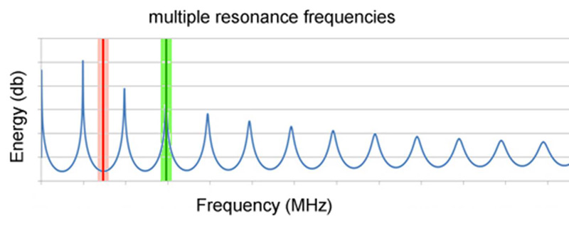
Fig. 7 shows an example of two selected measurement center frequencies with their respective bandwidths in a spectrum with resonances. The red center frequency will return only a small amount of energy from the cable system. Thus, the background noise will appear to be low but possible PD signals will also be very low. It is important to understand that the possible resonances in the frequency spectrum shown in Figs. 6 and 7 are the result of the aforementioned complex network of the chosen sensor, the physical location of the sensor, and the cable system under test. Therefore, these frequencies cannot be determined before arriving on site. They can only be determined once the HFCTs are placed at the cable system in multiple joints.

Often, the available time planned for the commissioning test is limited and cable installers and the owner push for rapid completion of the test. Moreover, it is in the economic interest of many parties to finish testing quickly. This pushes testing engineers to limit the number of center frequencies used at each measurement point, such as a joint bay.

If the PD testing setup in combination with the cable under test has resonance frequencies that are powerful enough to limit the measurement of PD at certain test locations, it can be difficult for the test engineer to determine this. The best possibility is to inject powerful non-classic calibration signals at one end of the cable system, having a variety of rise-times, pulse widths and fall times, measure this calibration signal at all testing points, such as the joints.

However, with cables above a couple of kilometers in length, this will be difficult since long lengths of jointed cable circuits constitute a distributed network of impedances. Therefore, conventional PD measurement, including conventional calibration, do not apply to measurement of PD on such circuits.

High Center vs Low Center Frequencies
The ability to detect calibration signals injected at one end of the cable is limited by attenuation of the signal, presence of noise and resonance frequencies of the cable system. Lower center frequencies (e.g. much below 3 MHz) allow for longer detection distances but this also increases amount of background noise. This is because both the PD signal and the background noise are attenuated by the cable. But the PD signal is attenuated more quickly – at least it seems that way. As a result, a PD signal becomes more difficult to distinguish from the background noise at lower center frequencies.

For center frequencies above 3 MHz or 4 MHz, the calibration signal can only be detected a few joints down the cable and in some cases even less depending on the design of the cable system. As a rule of thumb, the higher the center frequencies, the more localized the measurement will be around the test position (e.g. joint), thus reducing the “ability” of the HFCT to detect signals from larger distances.

Choosing higher center frequencies can be beneficial in the presence of high noise sources. Partial discharge from the HV source setup can be the origin of noise, especially if it cannot be mitigated properly. On long cables, these high center frequencies will make it difficult to detect the calibration signal over multiple joints and to ensure that any resonance frequencies in the setup are identified.

Selecting Proper Center Frequency
One way to ensure proper center frequency selection is to test at multiple joints simultaneously. This can be done by injecting a calibration signal through the HFCT at one joint bay and verifying that the signal can be detected at neighboring joint bays. The HFCT is positioned around the sheath cable at the link box in the same way that it will be positioned to test for PD. A wire loop from the calibrator is either threaded through the HFCT, as in the sensitivity check, or the HFCT is directly connected to the calibrator using a short 50 ohm coaxial cable.

If this procedure is repeated for different joints, the attenuation of the cable under test can be recorded for all center frequencies being used. This information can then be used to select the best center frequencies for PD testing. Of course, for such procedure multiple test teams need to work in parallel on neighboring joints.

It is important to note that PD testing on HV or EHV cable systems typically involves scanning for PD over a range of frequencies. This makes is easier to distinguish possible PD from noise source and localize these PD.

Voltage Source Setup
According to CIGRE TB 841 and TB 728, the cable system shall be without PD at 1.5 * U0 = 1.5 * 220kV = 330kV.
The used Resonance Test System (RTS) can energize a cable up to a testing voltage of 260 kV with a current of 70 A – 90 A. The longer the cable, the higher the capacitance. For longer cables, often 2 or more RTS need to be used in parallel to feed enough current to provide sufficient recharging current.

For cable tests above 260 kV, RTS need to be used in series, with the second reactor on insulators to reach voltage of around 520 kV. For this commissioning test, extra reactors are needed to elevate the voltage up to 330 kV, as required by CIGRE.
The RTS uses an adjustable frequency to tune to the resonance frequency in an LC network. The inductance (L) is part of the test system and the capacitance (C) is represented by the cable. Due to the cable’s length, the capacitance totals about 5000 nF, according to the specification sheet.

To drive enough current to energize the 22 km cable, four RTS units must be connected in parallel, with aforementioned extra reactors on insulating stands.

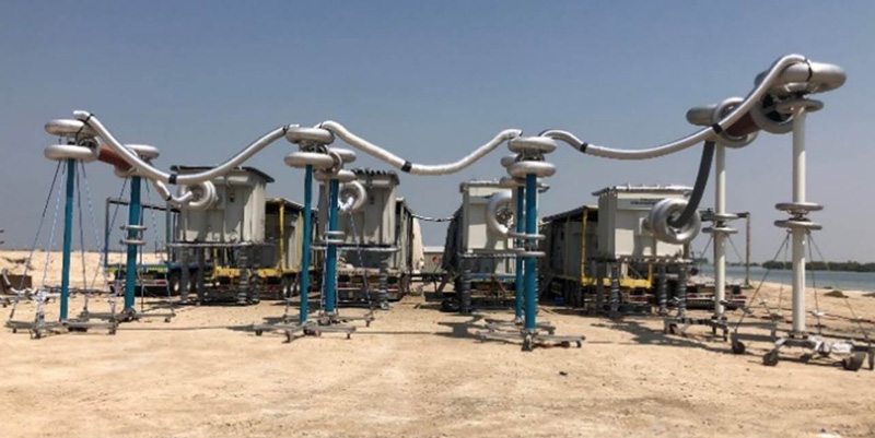
With 4 RTS and additional 4 reactors, the voltage source setup alone requires multiple technicians for minimum a day. The 4 RTS need to be synchronized with all voltage taps on the exciters being correctly set. This system needs to be connected to multiple diesel generators working synchronously as well to supply enough feeding power.

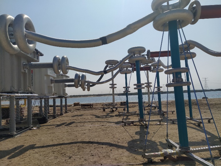
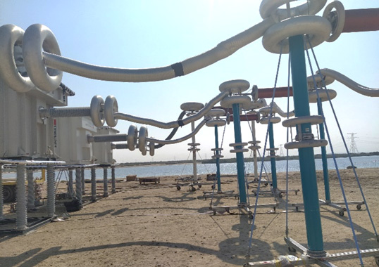
The HV connection from the voltage source to the test object is very challenging and takes multiple days to set up properly. A major challenge is the wind, which picks up sand and proximity to water. The combination of humidity, especially in the morning, and fine sand is highly challenging as dust settles on the conductors of the setup.

Due to the space required for the voltage systems, as well as the space needed to manoeuvre the trailers and diesel generators, in this case it was not possible to set up close enough to the cable under test. Instead, the setup was placed about 120 meters away, as shown in Fig. 10.

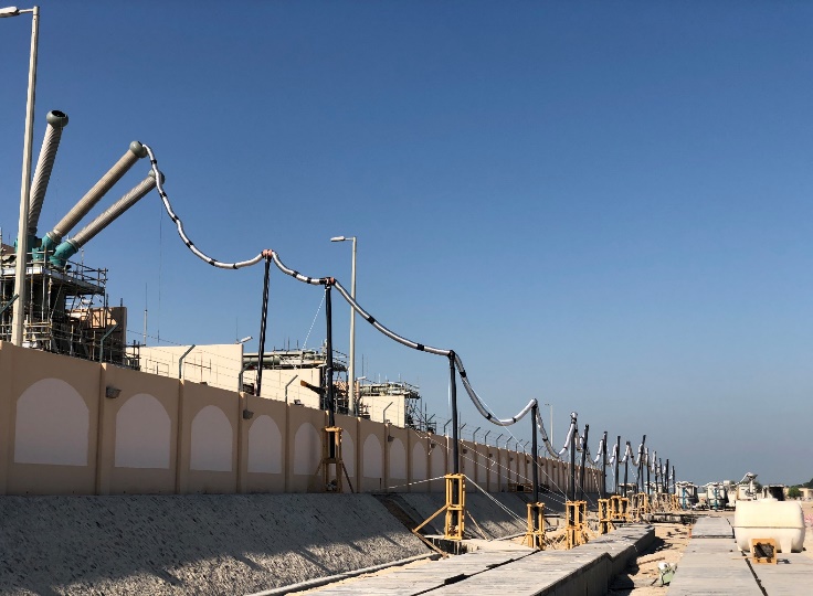
Under these conditions, it is economically difficult to create a setup that does not show any external discharges since this would take many days to set up and large investments in proper insulating stands. The current setup (Fig. 10) will result in PD during the measurement at the near end of the cable and thus properly interpreting the data requires expertise and skill. For the above testing project, the end client understood the issue and agreed to a commissioning test under these conditions.

Measurement Procedure

Testing a 33-joint-bay HV cable system with 2 end terminations can be a challenging task. One of the key challenges is that it is not feasible to test at all locations simultaneously. This is because fiber optic cables are not available to connect the joint bays. In this case, a ‘joint-hopping’ approach can be used

The following procedure was agreed upon with the end client:
– Perform a 1-hour withstand test.
– If the HV AC withstand test is successful, perform “joint-hopping” with 3 teams and energize for PD tests

This will expose the cable to a longer duration of energization above U0, but is more economical than deploying 35 PD measurement units with an operator each and testing them simultaneously.

In this joint-hopping approach, three teams are deployed to different joint bays. Each team is equipped with an HFCT, a calibrator, and a PD measurement device. The teams then connect their HFCTs in the link boxes and perform a sensitivity check at different center frequencies. After injecting calibration signals at the near end of the cable and at different joint bays, while measuring the calibrator signals at multiple joint bays simultaneously, the team decided to use 3 MHz and 8 MHz as the center frequencies, each with a bandwidth of 650 kHz.

The distance between the teams varied during testing since the cable was not along a single street. Instead, it crossed multiple streets, quarters and areas with varying levels of population and traffic. Mean distance between two joint bays was around 650 m, but the traveling distance from one joint bay to another could vary in the city from 3 minutes to over 1 hour, depending on routing and traffic.

Access to the joint bays was often next to roads and on sidewalks but sometimes on the road itself or in parking lots. Occasionally, cars were parked on top. If their owners could not be found within 15 minutes, the team would move on to the next joint bay. If at least two teams were ready to test PD at the joints, the cable was energized for about 5 minutes to 330 kV. During that time, one measurement was taken at 3 MHz and one at 8 MHz for a minimum of 1 minute each.

Measurement Results

Sensitivity Check
The sensitivity check was performed for 3 MHz and 8 MHz for all HFCTs by running a calibrator cable through the HFCT to determine the k factor. For both center frequencies and all HFCTs the k factor was around 5. This was expected, as the transfer function of the used HFCTs is almost linear in that area (see Fig. 4 as example).

Measurement of Partial Discharge (PD) Signals
The IEC 60270 standard defines how to calculate the charge value (Q) of repetitive partial discharges. The utilized measurement system shows the QIEC value for the last PDs in a screenshot. Usually, this value is used to describe the discharge values of PD or background noise respectively.

The sensitivity check does not constitute a calibration procedure according to IEC 60270 nor are chosen center frequencies of 3 MHz and 8 MHz within the recommended range. As such, the measured charge values will not be described as “QIEC” values. The measurement system calculates the charge by the same principle, but the value is called Q weighted (QWTD) instead.

Verification of Measurement Center Frequencies
One way to ensure that all possible PD in a cable system can be detected is to assure that sensors at each joint are able to detect signals from the respective adjacent joints if the signals are well above background noise. A calibrator signal with 100 pC was injected at three neighboring joints simultaneously, in this case joint bay 5, 6, and 7. The PD measurement at each joint was recorded.

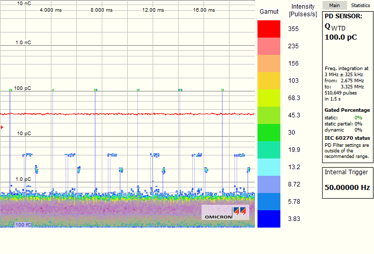
Fig. 11 shows the PRPD at joint 7. At 100 pC the calibrator signals from joint 7 can be seen as 6 dots within the 20ms time frame of the PRPD. This was the signal to determine the k factor. Also the calibrator signal from joint 6, around 650 m away, could be detected at around 4 pC, and the calibrator signal from joint 5, around 1300 m away, could be detected at around 1.8 pC. This shows that with the chosen measurement center frequencies it is possible to detect PD from adjacent joints, even over relatively long distances.

Figs. 12 and 13 show seven phase resolved partial discharge diagrams (PRPDs) each, from the end termination to joint 28, with both used center frequencies of 3 MHz and 8 MHz. The PRPDs show massive external discharges with different patterns, which were created by the long and disadvantageous HV source setup (as shown in Fig. 10). The external corona discharge signals are attenuated over distance, reducing the detectable and calculated charge value from joint to joint.

When utilizing a higher center frequency, a higher part of the signals frequency spectrum is measured. Especially on long cables, higher frequencies are attenuated more strongly than lower frequencies. This results in a stronger attenuation for the measurement with 8 MHz in relation to the measurement with 3 MHz.

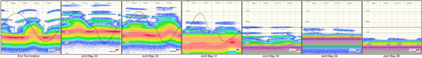
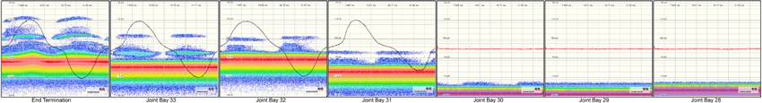
In Fig. 12 the corona discharges are still visible above background noise after 6 joints, around 3.9 km respectively. With 8 MHz, the corona discharges are barely visible after 4 joints, around 2.6 km.

In both cases, it is clear that the sensor at a certain joint is able to detect PD signals from adjacent joints, if the PD are well above background noise and of sufficiently low frequency content at the point of origin to propagate in a detectable manner to adjacent accessories.

In comparison with the calibrator signals in Fig. 11, one could assume that calibrator signals attenuate stronger than PD signals. The reason for this effect lies in the way, the calibrator signals were couples into the cable.
When a calibrator signal is injected into an HFCT, only part of the energy will couple into the cable screen. This already reduced energy will travel in both directions, roughly halving the energy again. This even smaller signal will be attenuated while traveling to the next joint, where it can be picked up by another HFCT.

Different signal propagation paths of PD signals within the cable system also explain the difference of the PRPD of the end termination and joint bay 33 in Figs. 11 and 12.

Part of the energy of the external corona discharge created at the HV setup will travel towards ground at the end termination. This part can be detected by the HFCT connected to the cable screen ground at the end termination. Based on the impedance of this ground, different parts of the signal’s spectrum behave differently.

The ”other” part of the corona discharge signals energy will travel “into” the cable and propagate along the cable to the adjacent joints and can be detected at the joint bays.

The different behaviour of propagation of different frequency contents gives the impression, that for 3 MHz the corona discharge is higher at Joint Bay 33 than at the end termination where the signals are created. This is not the case. The PRPD symbolize the split up of the discharge energy, with one part going directly to ground and the other part “into” the cable.

For 8 MHz, the discharge values at Joint Bay 33 show smaller values than for the end termination. Either a larger part of the relevant frequency spectrum travelled towards ground at the end termination, or the attenuation of that part of the frequency spectrum is already dominant enough to reduce the measured and calculated charge values at Joint Bay 33.

It is important to note that the energy levels associated with externally occurring corona are higher than those typically associated with internal PD occurring within an HV or EHV cable accessory. Signals created by internal PD will be less powerful and will not be visible over multiple joints and distances of over 3.9 km, at 3 MHz for this cable testing setup. Thus, it was not possible to assess, if internal PD occurred at the end termination and the first couple of joints. Testing from the other end of the cable was not feasible due to aforementioned reasons.

The future owner of the cables system was aware of the situation. Based on the fact that the cable system was energized well above U0 multiple times and was able to withstand the elevated voltage stress without failure, the cable was later tested with U0 and permanent monitoring for multiple days before being put into service.

Summary

Long cables do not behave like a lumped capacitance. As such, the calibration procedure according to IEC 60270 is not feasible. When testing PD on joints, the transfer function of the HFCT sensor used do not represent the frequency response of the full PD measurement setup.

The full PD measurement setup, a combination of the cable under test + the sensors + leads to the sensor + location of the sensors creates a complex network of impedances. These impedances are cause for a unique signal response.

Measurement center frequencies can not be pre-selected but must be determined at site to assure in a cross-check, that PD signals, or at least calibrator signals, from adjacent joints can be detected.

Joint hopping can be a form of testing long cables. This should be executed by multiple teams at the same time to perform the cross-check.

PD signals will attenuate over distance travelled in the cable. The higher the chosen measurement center frequency, the higher the observed attenuation of signals.

References
[1] CIGRE TB 728, May 2018, B1 Technical Brochure: “On-site Partial Discharge assessment of HV and EHV cable systems “, WG B1.38
[2] CIGRE TB 841, Sept. 2021, B1 Technical Brochure: “After laying tests on AC and DC cable systems with new technologies”, WG B1.38
[3] IEC 60270, 2015, “High-voltage test techniques – Partial discharge measurements”
[4] IEC 62067, 2006, “Power Cables Above 150 kV and their Accessories for Rated Voltages Above 150 kV (Um = 170 kV) up to 500 kV (Um = 550 kV) – Test methods and requirements”
[5] M. Fenger J. Levine, “Sensitivity Assessment for HV & EHV Field Partial Discharge Measurements via Laboratory Testing”, IEEE Conference Record of the 2008 International Symposium on Electrical Insulation, June 2012 
”
[6] N. Oussalah, Y. Zebboudj & S. A Boggs, “Partial Discharge Pulse Propagation in Shielded Power Cable and Implications for Detection Sensitivity”, IEEE Electrical Magazine, Vol 23. Issue 6, pp.. 5 – 10, Nov/Dec 2007.

[inline_ad_block]