In typical electrical systems, the capacitance between multiple conductors is of primary interest and to facilitate such calculations it is possible to arrange the mutual capacitances of a system of N conductors into a matrix format. ELECTRO and COULOMB programs can then prove invaluable for precise calculations of capacitance matrices in electrical systems. Below are examples to illustrate this, as prepared by Dr. K.M Prasad, Senior R&D Engineer at Integrated Engineering Software

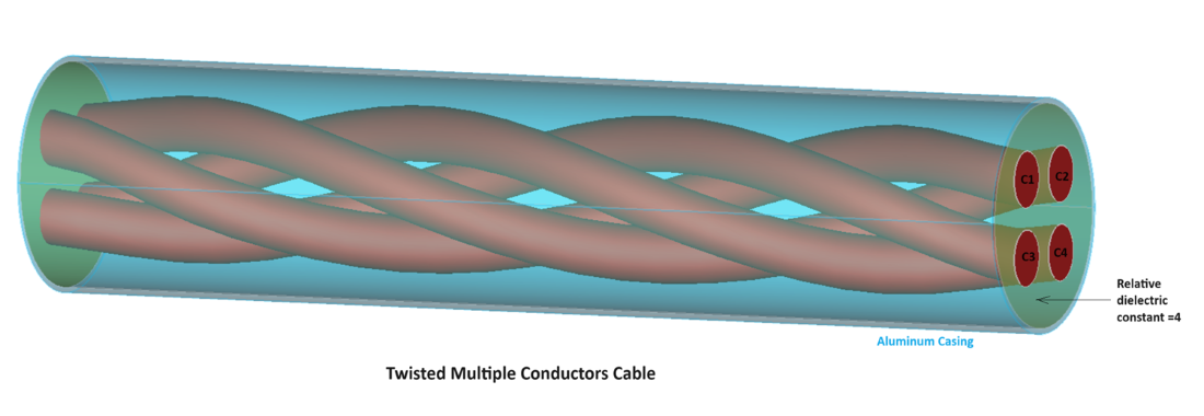
For computation of the capacitance matrix in a twisted multiple cable model and to speed up the solution process, the symmetric and periodicity set-up feature in 3D Electric Field Solver COULOMB proves especially useful. The image below, for example, shows four conductors embedded in a dielectric material with εr = 4. Each conductor has a radius of 5 mm within a cylindrical shaped cable of radius 20mm (see Image 1).
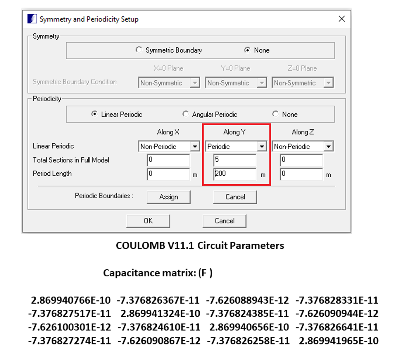
For a one-meter length of cable, computation of the capacitance matrix can require approximately 5 to 10 minutes because of the large aspect ratio between the radii of the conductors and their length. To address this issue, an analysis was conducted using a 200 mm length cable centrally located at the point (0,0,0). The number of sections used in the Linear Periodic Condition was 5. Around 10,000 2D triangular surface elements were used to solve the model. COULOMB efficiently solved the model in just 85 seconds utilizing 118 MB of RAM. Image 2 shows the resulting capacitance matrix for this model.
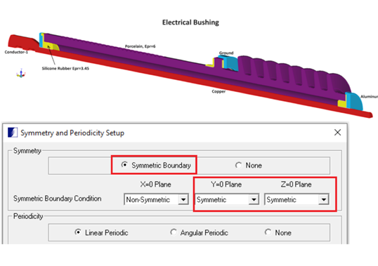
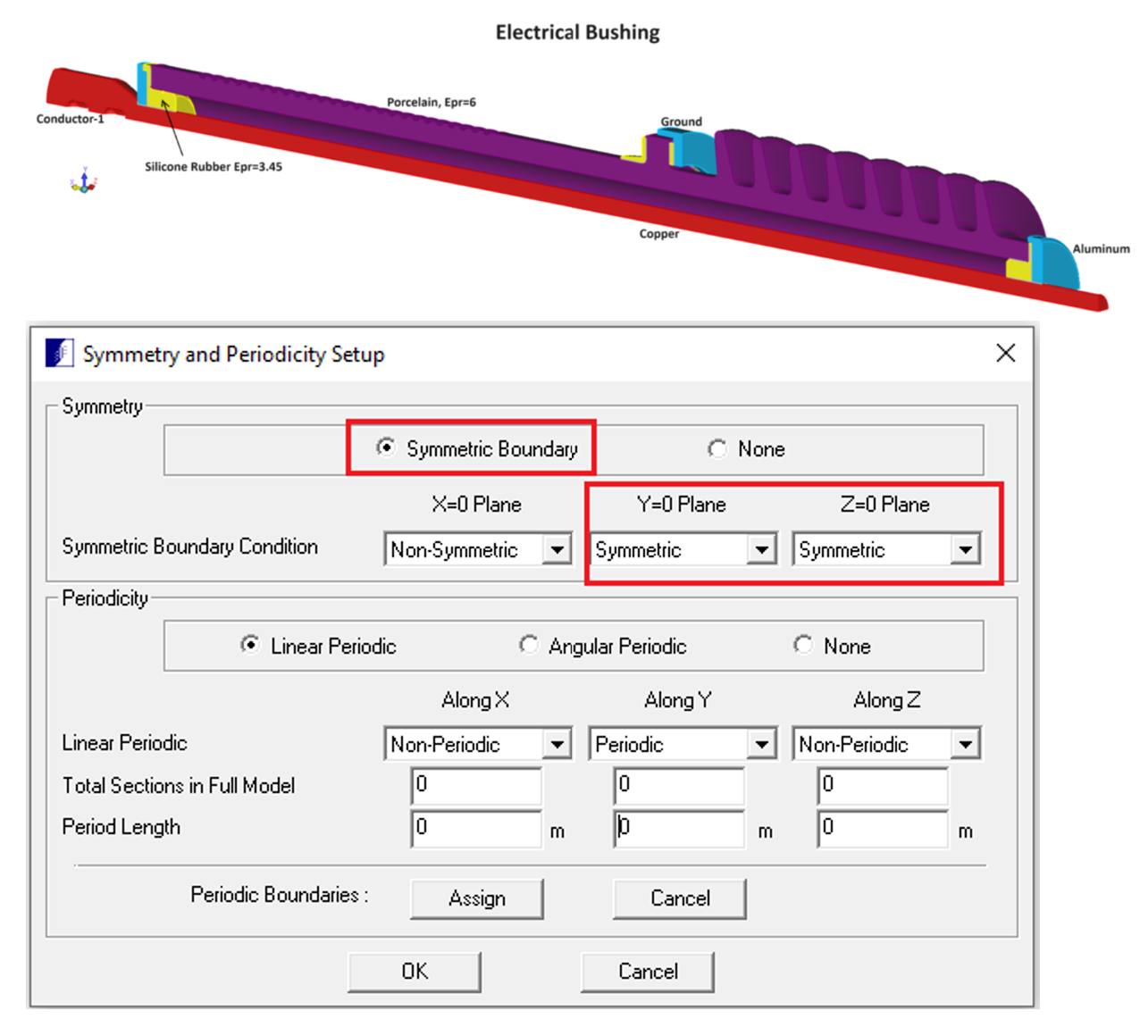
Similarly, an electrical bushing model was also solved using COULOMB with symmetric conditions applied along y=0 and z=0 planes which effectively simplified the model by 4 fold, as seen in Image 3. Capacitance calculations were performed between Conductor-1 and Ground resulting in a capacitance value of C11= 3.086301222E-11 (F).
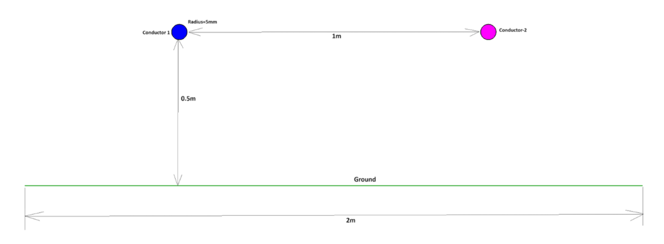
ELECTRO applied the Boundary Element Method to compute the capacitance matrix in the electric power line model shown in Image 4. The elements in the capacitance matrix were calculated as follows:
The first column of the capacitance matrix was calculated by applying 1V to Conductor 1 and 0V to Conductor 2 and grounding. This yielded C11 = Q1/1V = 1.468076963E-11 F and C21= -Q2/1V = -1.831800433E-12 F, where C21 is called the mutual capacitance between Conductor 1 and Conductor 2. The partial capacitance of Conductor 1 with Ground is the algebraic sum of C11+C21 = 1.468076963E-11 F – 1.831800433E-12 F = 1.28489692E-11 F.
Similarly, the second column of the capacitance matrix is calculated by assigning 1V to the Conductor 2 and 0V to the Conductor 1, while maintaining the Ground at 0V. Since this model is a symmetric model, C22=C11. In this model, there are no dielectric materials. Hence, the Free-space Capacitance matrix is the same as the Capacitance matrix.
If dielectric materials were present, ELECTRO would re-compute the model by replacing the dielectric materials with free-space and calculating the free-space capacitance matrix.