Often, overhead groundwires (OHGW) are among the first components to fail on overhead transmission lines. OHGW end-of-life assessment often triggers a mid-life renovation project to ensure many more years of reliable service from an overhead line in a desirable right-of-way.
This edited contribution to INMR by Dr. William Chisholm, in co-operation with Kinectrics, proposes a process to review and quantify the performance of OHGW systems to rank possible renovation options. In some cases, these should consider replacing OHGW protection with other components, including optical fiber ground wire (OPGW) installed below the phases. With suitable arresters, this underbuilt OPGW can be energized at modest voltage to support future monitoring of infrastructure.
Rebuilding / Refurbishing Project Resources
One of the aspects in reviewing a resource from 1955 (Ohio Brass Company, 1955) is that many of our “modern” new approaches to improving lightning performance have many decades of experience. However, modern technology also allows us to test long-term perceptions that electrical attachment of lightning to power lines is the root cause of all tripouts and faults during thunderstorms.
Improved Classification of Outage Root Causes
Lighting performance scales linearly with Ng, in every estimating method. There is an implicit assumption that the lightning parameters such as median peak current do not change with location. Based on previous experience, there is a second assumption that the lightning activity in the decades after completing a project will be the same as the density in the past.
Thunder Activity
Records of thunder have been available in some regions for 1000 years, but the link between thunder activity and cloud-to-ground lightning flash density is weak (IEEE Power & Energy Society, Transmission and Distribution Committee, 2011 Jan 28) (CIGRE WG C4.23, June 2021). Some storms have a high fraction of intra-cloud or inter-cloud activity that never reaches the ground. Others, for example frontal storms in winter, sweep through areas and deliver a high fraction of positive-polarity flashes with exceptional charge compared to the usual strokes in a negative-polarity flash. In 1991 (CIGRE WG 33.01, 1991), CIGRE recommended a relation of Ng = 0.04 TD1.25 but removed this recommendation in 2021 (CIGRE WG 33.01, October1991 revised 2021).
Lightning Flash Counters
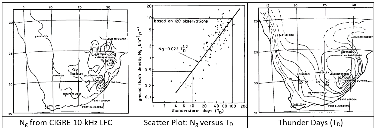
In the 1970s and 1980s, work in South Africa (Anderson, Niekerk, Hroninger, & Meal, March 1984) and CIGRE led to improved electronic lightning flash counters that responded mainly to ground flashes. These sensors measured the change in vertical electric field above a threshold, after matched filtering. Calibrations showed a 10-kHz center frequency gave 20-km range. Flashes were tallied with mechanical counters that advanced once per second. Multiple ground terminations and subsequent strokes within 1 s were automatically grouped as a single flash to ground. There is a general trend in Figure 2 for areas with more thunder to have more lightning to ground, but a region with TD = 40 days in the scatter plot might have 1 < Ng < 5.
The CIGRE LFC proved to be an excellent resource for discriminating legitimate lightning flashes from other faults, considering the service area of a single distribution station (DS). This approach worked best when the monitoring system captured the simultaneous records of fault current and LFC operation. For longer transmission lines, a single LFC does not have the range to capture all the lightning activity.
Ground-Based Lightning Location Networks
Initially based on direction finding, receivers that are also synchronized in time using global positioning system satellites have been the primary tool for lightning investigations for two decades. A total of 200 sensors are located throughout Canada and the USA.
Lightning location systems (LLS) serve as a fundamental resource to establish the appropriate priority for modifications. There is no point, for example, in fitting overhead groundwires or arresters, if studies of observed faults have not found agreement – to the millisecond – between the observed times of tripouts and the times of recorded strokes to ground. Ten years ago, lightning was cited as the root cause of more than half of all transmission outages. With the use of precise data from LLS, reports to NERC now suggest that “unknown” outages are more frequent than lightning. This gives more priority to controlling the motion of conductors – or assessing the other root causes of outages during adverse weather – through better exploitation of time-coincidence studies.

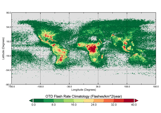
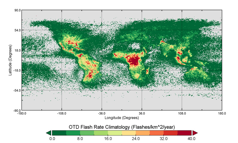
Optical Transient Detector Satellites
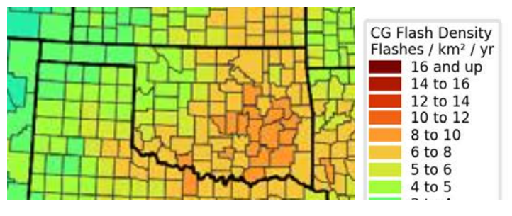
In 1997, NASA initiated a series of instruments that monitored the number of optical transients from outer space. The optical transients are a mix of cloud and ground flashes. The grouping algorithm of pixels to flashes used in Fig. 3 now considers the large physical extent of some flashes (Peterson, Mach, & Buechler, 19 Feb 2021). Recent lightning protection guides (IEEE Power & Energy Society, Transmission and Distribution Committee, 2011 Jan 28) (CIGRE WG C4.23, June 2021) recommend that, in places with no LFC or LLS, Ng should be estimated from the long-term observation of OTD, divided by a conversion factor of 4 ± 1 (CIGRE WG C4.23, June 2021). IEEE (IEEE Power & Energy Society, Transmission and Distribution Committee, 2011 Jan 28) provided plots using a factor of 3, so that Ng = OTD/3. This factor was also used in Fig. 4. There is considerable scatter between reference LLS data and OTD data because the OTD observations were taken in a region above 49° north latitude, not monitored by the subsequent LIS instrument, and the number of observations in each grid square is small.
Since 2017, a new LIS instrument has been reporting lightning data from the International Space Center (ISS), covering latitude of ±55°. Also, the Geostationary Lightning Mapper (GLM) has been operating on the GOES-East and GOES-West satellites, with real-time data presentation at (NOAA, 2023). These satellite observations can be compared with real-time lightning maps from a “citizen science” project at Blitzortung.org.
Intercomparison of LFC, LLS & Total Lightning Activity
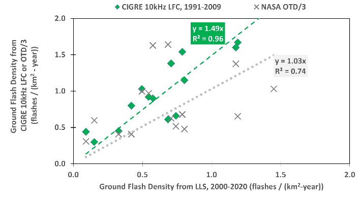
Fig. 4 compares readings of Ng from CIGRE 10-kHz lightning flash counters in the Canadian province of Saskatchewan, 1991-2009, and optical transient density (OTD) estimates from the NASA OTD project, with twenty years of observations from the NALDN Lightning Detection Network (Environment Canada, 2016). The linear regression between the CIGRE LFC and NALDN LLS results in Fig. 4 is strong but there is a slope error of about 50% – the LFC suggest a higher Ng than the LLS.
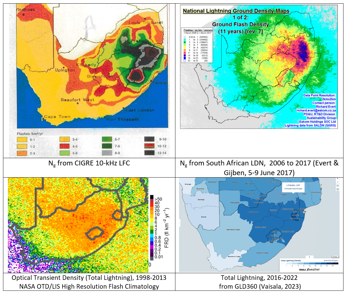
Results of ground-flash and total event density In South Africa are compared in Fig. 5. All data sources show a strong gradient in lightning activity, low in the west and peaking at 30°W, 30°S in Ng observations, whether using a network of 400 LFC (Anderson, Niekerk, Hroninger, & Meal, March 1984), a 25-sensor LLS within South Africa (Evert & Gijben, 5-9 June 2017), a satellite-based optical transient detector of total lightning activity, and one of the global ground-based LLS that use multiple reflections from the earth-ionosphere waveguide, also to provide total lightning density (Vaisala, 2023).
The South African experience was that there were large regions in the east with Ng > 14 flashes/(km2-yr) in the LLS data, compared to no regions with Ng > 14 from the CIGRE 10-kHz LFC. This differs from the LFC-to-NALDN comparison in Figure 4 for an area with low flash density.
The latest innovations in lightning detection make it possible to resolve multiple ground-termination points that have been measured using photographs and video systems for many years. An estimate of the number of “true” ground termination points in (CIGRE WG C4.407, August 2013) is that there are 1.5 to 1.7 channel terminations on ground per recorded flash location.
Correction of Attractive Radius When Using Ng from LLS
Predictions of lightning performance apply models of the attractive radius, based on conductor height at the tower (IEEE, September 2008), (IEEE Power & Energy Society, Transmission and Distribution Committee, 2011 Jan 28) or a “lateral attractive distance” (CIGRE WG C4.23, June 2021) based on average conductor height. These models were all calibrated to match the observed number of flashes to an 11-m test line in an area of South Africa where Ng was established using lightning flash counters. Observed outage rates in other regions can be used, along with locally observed Ng, to confirm the effective capture width. For South Africa, the number of flashes to an unshielded single-conductor line, # = 2.8 Ng ht0.6 with height at the tower ht in meters (IEEE, September 2008) (IEEE Power & Energy Society, Transmission and Distribution Committee, 2011 Jan 28) (CIGRE WG 33.01, October1991 revised 2021), with Ng measured with a CIGRE 10-kHz LFC. When Ng is obtained instead from the South African LLS (Evert & Gijben, 5-9 June 2017), perhaps the estimate of # should be adjusted to (2.8 x 14/18) = 2.2 Ng ht0.6, where 14 and 18 are the highest values of Ng from LFC and LLS observations in Fig. 5.
Unshielded Line Performance Analysis
There are other lines that can be used to confirm the models of lateral attractive distance. These generally are the long, unshielded transmission lines, often located in rugged terrain and perhaps in climate with heavy icing conditions. It is expected that nearly every stroke to an unshielded transmission line will cause a line-to-ground flashover. The stroke current flows into the surge impedance of the phase, in two directions and even for bundle conductors, insulated with 3-m dry arc distance, it only takes less than 10 kA to cause a flashover in the usual direction, from energized conductor to ground. More than 95% of the first negative return strokes (median 31 kA) will exceed this current level. Even if the first return stroke is weak, one of the subsequent strokes may exceed the median of 12 kA. Thus, the lightning performance of an unshielded transmission line is a faithful indicator of the number of flashes that terminated on that line.
Several of the case studies in (Ohio Brass Company, 1955) describe projects where unsatisfactory lightning performance of an unshielded transmission line led to a rebuilding project.
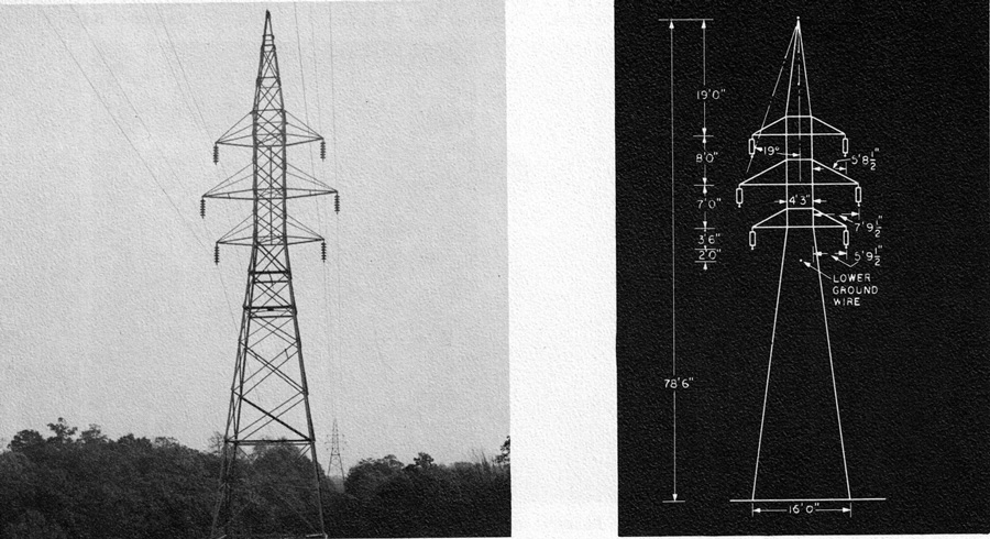
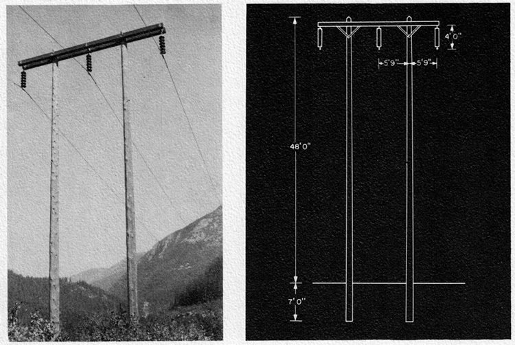
A 69 kV transmission line in Weleetka, Oklahoma (35.3° N, 96.1°W) reported an annual outage rate of 47 per 100 km-yr prior to installing twin OHGW. This line used wood H-frame construction with phase spacing of 3.2 m. Using an estimate of Ng = 8 flashes/(km2-yr) for this region, the attractive width of the line w, based on 19 years of observations, was (IEEE, September 2008):
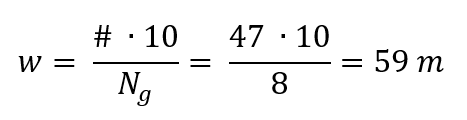
The 1955 blueprint for this line shows a phase conductor height at the tower of 12.1 m. Using the overall phase conductor width of 6.4 m, the estimated w from (IEEE, September 2008) is 131 m. The discrepancy between calculation and observation is usually attributed to the benefits of environmental shielding from trees along the right-of-way, illustrated in Fig. 7.
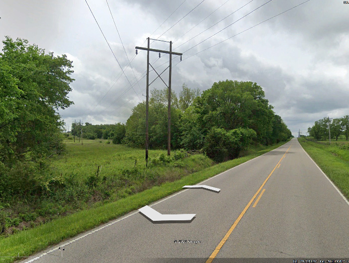
It is possible to invert the model to estimate the average height of the phase conductors above the average tree height but every span has a different exposure. After installation of OHGW, like those in Figure 7, the outage rate fell to 5.2 per 100 km-yr. This did not quite achieve Class-C reliability, but the performance is rather good for this voltage level, considering the high level of lightning activity. There are several other similar case studies in (Ohio Brass Company, 1955), showing the efficiency of OHGW installation with before- and after-treatment outage rates.
Unshielded Line with Externally Gapped Protector Tubes (EGLA)
In 1943, New York State Electric & Gas Company constructed a 42.8 km transmission line at 114 kV, using seven standard 146 x 254mm disc insulators. In contrast to the usual practice, this line placed “protector tubes” vertically below each phase, on a thin 24’ crossarm.
The protector tubes were known even in the 1930s (Sporn, June 1933) but did not become a practical “current limiting gap” alternative to metal oxide surge arresters until 2005 (CIGRE WG C4.39, December 2021). In this application, the observed lightning outage rate was 2 faults per 100 km per yr, meeting “Class C” reliability typical for this voltage class. The lightweight crossarm supporting the thin, hollow protector tubes from below is an attractive and practical arrangement, especially compared to hanging the same device at an angle from the upper crossarm. The tendency for protector tubes to be longer than the protected insulator strings is present today for TLSA applications on system voltage of 275 kV or higher. Davit arms can also intercept a conductor if there is a hardware or insulator failure, so these are seen on some urban transmission lines.

Unshielded Line with Non-Gapped Line Arresters
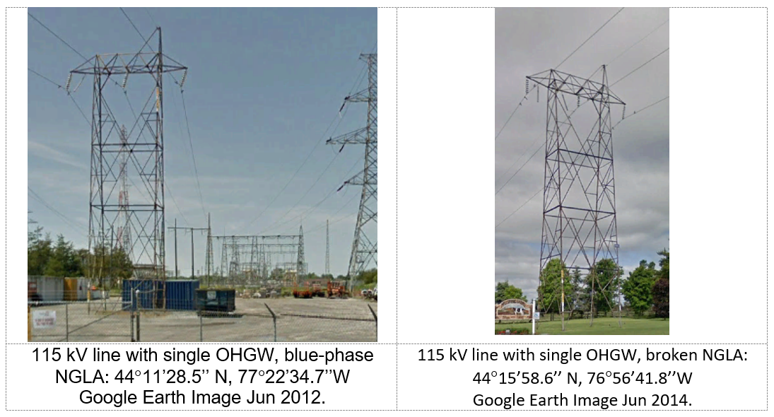
The Hydro-One transmission network in Ontario, Canada developed over a long period of time and consists of a wide range of structure designs. Material shortages during WWII led to the construction of 115 kV lines with one rather that two OHGW, as shown in Fig. 9. The missing OHGW leaves the blue phase exposed to direct lightning flashes. These towers had a typical height of 22.4 m at the OHGW peak. With seven standard disc insulators the OHGW gave shield angles of 26, 31 and 59 to the red, white, and blue phases respectively.
Customer requirements for a reduction in momentary outages led to a co-funded project to improve the lightning performance of this line. Based on the age of the structures, the utility was reluctant to install a second OHGW to protect the blue phase. Evaluations (Tarasiewicz, Rimmer, & Morched, July 2000) in Fig. 9 ranked relative performance, predicted outage rate relative to observed long-term value of 2.23 outages per 100 km per yr, against the cost relative to fitting non-gapped line arresters (NGLA) across every insulator.
Fitting a second OHGW would have cost 78% of the cost of installing 398 arresters on this 98-km line. It was predicted that installing arresters on all exposed (blue) phases, and on all three phases at 22% of towers with high footing resistance, would give a 95% reduction in lightning outage rate at 44% of the cost of full arrester treatment. This was the option selected.
Energy duty for arresters on unshielded phases was computed to be about 1700 kJ for a 200-kA peak current to mid-span. Arresters with 84 kV maximum continuous operating voltage (MCOV) and 185 kJ energy rating were selected with a view to achieving an arrester failure rate of 0.07% per year. These arresters were equipped with explosive disconnectors in the ground leads to isolate failures.
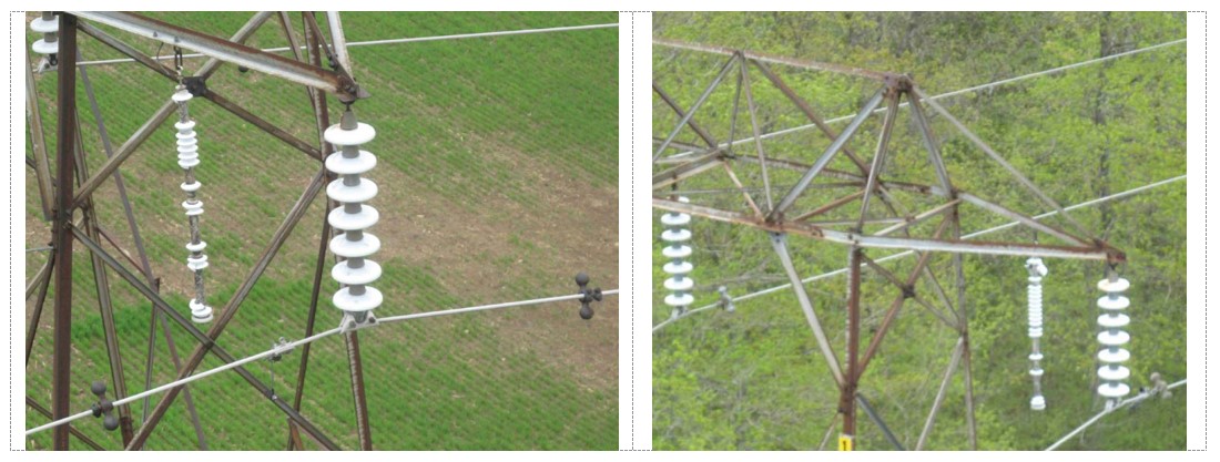
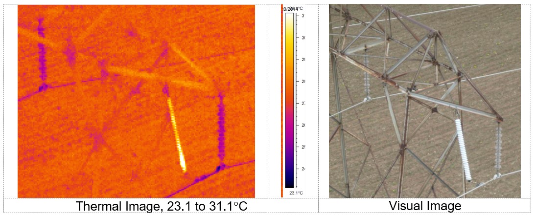
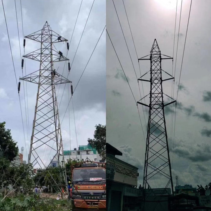
There were a series of mechanical problems with the arrester installations, with each mounting arrangement providing about seven years of reliable service. For example, the right-hand photo in Fig. 10 shows the blue-phase arrester hanging vertically, indicating a broken disconnect wire. The central (white) phase arrester remains at its proper angle. The red phase arrester is missing completely. Diagnostic testing showed arresters removed from the tower were intact, but fatigue damage to flexible lead wires had broken the connections to phases. The 2014 images in Fig. 10 signaled that this arrester project was reaching its end of life. Helicopter inspections that year turned up an increasing number of failed arresters (Fig. 11) as well as arresters that were running warm based on thermal inspection (Fig. 12).
The co-operating customer who paid for the arresters originally under a performance contract ceased operations in 2009. By 2023, all NGLA installed in 1997 have been removed, restoring the line to its original poorly shielded configuration. Overall, this utility maintained a momentary interruption rate of 0.54 dips per year in 2009-2018, added to 0.6 sustained interruptions per delivery point per year.
Simplified Backflashover Model Based on Fixed Ramp Time of 2 μs
Backflashover calculations are normally carried out with the parameters of the first negative return stroke (CIGRE WG C4.407, August 2013), because these have the largest values of Ipk that tend to give the highest levels of Vpk using Fig. 13.
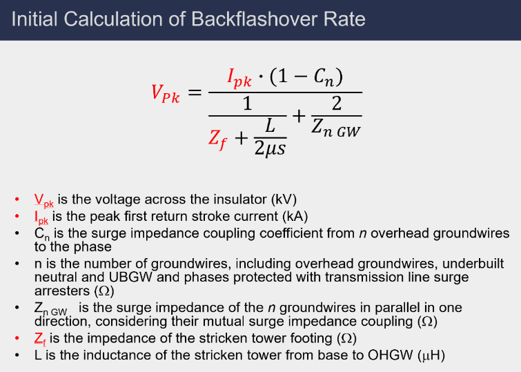
There is no single value for Ipk. Instead, it is described by a log-normal statistical distribution, with median 31 kA and standard deviation of ln(Ipk) between 0.48 (CIGRE WG 33.01, October1991 revised 2021) and 0.66 (IEEE, September 2008) (Takami & Okabe, January 2007). The tower footing impedance Zf in Fig. 13 also has a log-normal distribution. The log standard deviation of resistivity, based on 300-m distance between sites, has been found to be in the range of 0.9 (Chisholm & de Almeida de Graaff, Adapting the Statistics of Soil Properties into Existing and Future Lightning Protection Standards and Guides, 28 September – 2 October 2015) for regions in the USA and Portugal. The distribution of Vpk, computed in Fig. 13 is thus the product of two very wide statistical distributions. Failure is always an option, and we are engineering instead to a desired failure rate specification, such as the Class A/B/C requirements listed above.
Usually, the insulation strength is well known, so the process is inverted to compute the critical peak value Icrit that equates V¬¬pk with this strength. This is done for the expected range of values of Zf. Then, the probability of receiving a first return stroke exceeding Icrit is established by inverting its log-normal distribution, using an Excel LOGNORM,DIST function or estimate P (i>I) ≅ 1/(1 + (I/31 kA)^2.6).
Fig. 13 fixes the zero-to-100% rise time of 2 μs and uses it to convert tower inductance to voltage rise, using the model ΔV = L dI/dt = LI/(2 μs). The voltage rise at tower top is the sum of footing voltage rise Zf •I and L dI/dt. The voltage rise at intermediate positions along the tower is established by the current flow and the inductance from that point to the ground. This is often scaled linearly if the tower has a cone shape, like a steel monopole, with constant surge impedance viewed from the apex.
It turns out that the original choice of a linear ramp wave with zero to peak time of 2 microseconds (2 μs) (EPRI, 1982) remains an excellent choice for evaluating the overvoltage that appears across insulators under lightning surge conditions. Measured downward negative first return strokes generally have a concave front that reaches its maximum derivative Smax, dI/dt just at the peak of the current wave (CIGRE WG 33.01, October1991 revised 2021) (CIGRE WG C4.407, August 2013). The equivalent ramp front time, extrapolating back from peak at the rate of Smax to zero current, seems to increase slowly in the range of 1.8 to 2.5 μs, depending on peak current magnitude.
References describe several adjustments to the simple model in Fig. 13:
• The volt-time curve for impulse flashover: often a calculation is done for time to flashover in the range of 1 to 3 microseconds, and the evaluation time depends on span length;
• The surge impedance coupling from those OHGW, faulted and arrester-protected conductors that carry a fraction of the lightning surge current away in each direction from tower top;
• The additional voltage rise associated with fast-rising current flow in the inductance of the thin monopole structure;
• The variability of soil resistivity and footing impedance from structure to structure;
• The effects of corona, which absorbs energy from the lightning and reduces stress on the insulators;
• The effects of line voltage, as one phase will always have an instantaneous voltage that adds to the stress;
• The effects of line surge arresters on the distribution circuit, which convert protected phases to extra groundwires and thus provide some benefits even to the unprotected transmission phases above.
An initial calculation will compare results using a fixed value of footing resistance at each tower, incorporating a volt-time curve, surge impedance coupling and tower inductance. The computed value of Icrit, and the probability of exceeding it, will then be compared to a composite result based on a realistic log-normal distribution of soil resistivity that changes from tower to tower. The effects of impulse corona on Icrit will be demonstrated for the transmission circuit, with and without the distribution underbuild to show the improvement in coupling. A new model for the coupling and wire surge impedance is demonstrated. At the assumed transmission and distribution system voltage levels (115 kV and 50 kV), power system voltage bias is not as important, but it does reduce Icrit slightly, increasing the backflashover rate by a factor of about 20%, independent of footing impedance. The surge impedance matrix is used to estimate the currents that will flow through each surge arrester placed in parallel with distribution system insulators. Based on these currents, the voltage drops across the arresters can then be subtracted from the voltages on protected phases to re-assess the voltages that will appear on unprotected transmission phases.
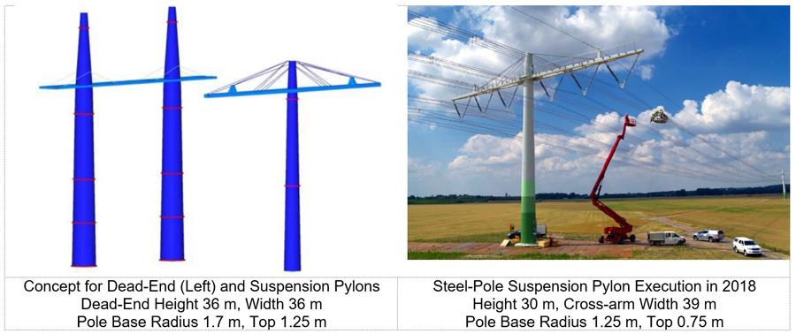
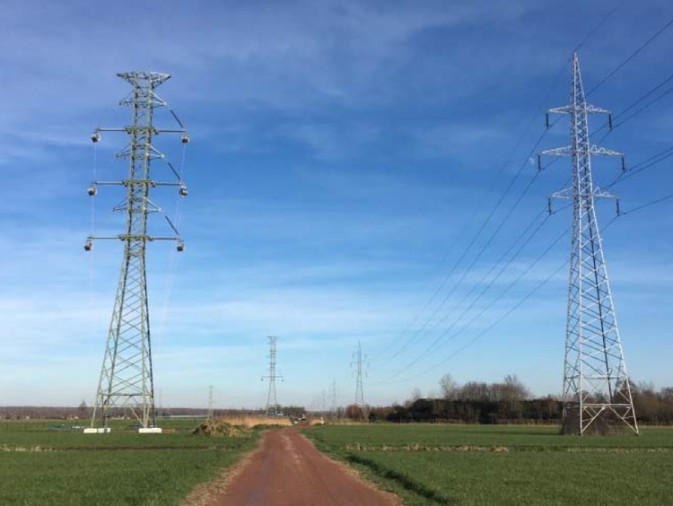
CIGRE Technical Brochure 792 (CIGRE WG B2.63, February 2020) discusses the substitution of conical solid-wall steel pylons for lattice steel structures to support higher tensile force on crossarms and to reduce the footprint at tower base to a single, large foundation. This set of choices affects lightning performance in several ways. The pylons described as a case study in (CIGRE WG B2.63, February 2020) and the simplifed model in Fig. 13 serve to illustrate the various issues.

A compact transmission line design with double-circuit V strings in Fig. 14 restrains the horizontal motion of conductors, which is fundamental to a successful design. When V-strings are used, the dry arc distance from the conductor to crossam is reduced, for example with insulators at 45° angle, by a factor of √2. The dry arc distances from conductor to tower establishes the maximum VPk in Fig. 13.
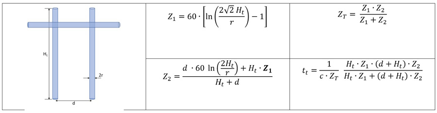
The pylons in Fig. 14 have two overhead groundwires. On the suspension plyons, these are located on 2-m vertical horns above the crossarm at height 25 m, each placed 12 m away from the vertical conincal section. Considering a stroke entering the tower at one of the OHGW attachments, there is an additional 14 m of path length, and 12 m of this path length adds to insulator stress. With a crossarm geometric radius of about 0.2 m, the surge impedance of the arm is Z = 60 ln (2h/r) = 60 ln (2×25/0.2) = 331 Ω, and its travel time is (12 m / 3×10⁸¬ m/s) = 40 ns. The inductance of the path from base of OHGW attachment to the tower is L = τZ = (40 ns)(331 Ω) = 13 μH. With the model in Fig. 13, this extra inductance from the base of the insulator to the base of the tower adds a voltage rise of (13 μH/2 μs) = 6.5 V/A to Vpk. Considering a severe lightning return stroke current of 100 kA, the voltage drop along the crossarm will be 650 kV. The impulse voltage on the outer four phases will be higher than the middle two phases, and for balance would need an additional 0.8 m of dry arc distance.
The additional inductance of the path length along the suspension pylon crossarm in Fig. 14 is mitigated by the presence of railings and guy wires. The guy wires are attractive but the railings detract from the clean visual appearance. However, both metal elements carry some lightning surge current, and combine to form a relatively large geometric mean radius – 1 m rather than 0.2 m for the crossarm alone. Additional details on models that include crossarms in estimation of tower surge impedance and inductance are found in (CIGRE WG C4.23, June 2021).
The surge impedance of the conical tower body from crossarm to ground is calculated using the same expression, Z = 60 ln (2h/r). The average impedances in Table 1 use slices of the pylons every 5 m.
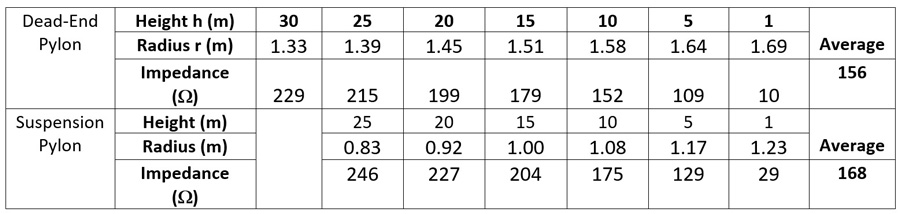
The surge impedance formula behaves badly when height is small, but measurements show that using h = 1 m in Table 1 rather than h = 0 gives realistic results. Only the portion of the pylon from the crossarm to ground is considered in the calculations. As was the case for the calculation of crossarm inductance, the travel times τ are the lengths of these sections, divided by the speed of light c.
There is a second advantage to the H-shaped configuration of the dead-end tower in Fig. 14. There are two, rather than one, vertical pylons. While it might be expected that the impedance of two pylons in parallel is half of a single pylon, ZT = 156/2 = 78 Ω, there is mutual surge impedance coupling between the two sections. According to the corrected calculation process in (CIGRE WG C4.23, June 2021), the portal structure has an impedance ZT = 100 Ω and average travel time of tt = 145 ns, giving an inductance of L =14.5 μH.
The impedance of the stricken tower footing Zf depends on the size and shape of the buried portion of the tower. For a monopole, the depth of burial is commonly estimated as at least 10% of the pole length, plus 0.6 m. Pole heights and burial depths are relatively constant along a line section.
Backflashover Model with Arresters
Surge arresters, placed across the insulators, will limit the local overvoltage as they pass a fraction of current into the protected phase conductors. This has the desirable feature of increasing n, the number of groundwires, in Fig. 13. It will also affect the coupling coefficient, which was fixed at Cn=0.3 in Fig. 13 to focus on the role of log-normally distributed soil resistivity. The process to compute the values of Cn for each phase is complicated and important enough to merit its own section.
Modeling of Surge Impedance Coupling in Excel
Most of the simplified programs for computing lightning performance (EPRI, 1982) (CIGRE WG 33.01, October1991 revised 2021) (Hileman, 1999) (EPRI, December 2005) (EPRI, 2008) (EPRI, 2004. 1002021) have some limitations with regard to the number of circuits and groundwires. In 2019, a spreadsheet (Chisholm W. A., Arrester Protection of Lower Voltage Circuits on Multi-Voltage Towers: Issues & Opportunities, October 20-23, 2019) was used to model the effects of six additional groundwires on a mixed four-circuit transmission and distribution line in Fig. 15.
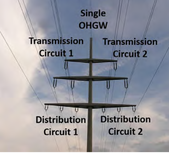
While there is only a single central OHGW, applying LSA to the bottom six conductors brings them into a 13-wire surge impedance coupling circuit. This is visualized first with a linear model that can be verified in experiments. Then, the effects of impulse corona on the surge impedance and coupling matrix are explored. Finally, the effect of line voltage and voltage drops across the arresters was evaluated. For convenience, details of this work are reproduced from (Chisholm W. A., Arrester Protection of Lower Voltage Circuits on Multi-Voltage Towers: Issues & Opportunities, October 20-23, 2019). Then, the influence of a new model for impulse corona (Rizk, Negative Impulse Ground Wire Corona Parameters for Backflash Evaluation of High Voltage Transmission Lines, August 2022) is evaluated to provide a second perspective on the advantages of “embedded ground conductors” located within the transmission circuits (Rizk, Novel Solution to Back Flashovers on High Voltage Transmission Lines: The Embedded Ground Conductor, December 2022).
The concept of placing a ground wire below or among the phases is not new. For example, Duquesne Light Company added a second groundwire at a height of 39’ (11.9 m) “to increase the coupling effect” in 1941. The merits of UBGW for a double-circuit 345 kV transmission line were mentioned in IEEE Standard 1243-1997 (IEEE, September 2008), and show that placing one or two UBGW inside the phase conductors gives the greatest reduction in backflashover rate.
Engineering is needed to ensure that any UBGW does not contact or intrude on electrical clearances to phase conductors. For the Duquesne design, the UBGW was tensioned to prevent contact at wind speeds up to 97 km/h on un-iced conductors with typical span length 630’ (192 m).
Self and Mutual Surge Impedance Matrix
Impedance of a conductor over ground at power frequency is a complex number, but as the frequency f increases from 50-60 Hz to over 100 kHz, the series resistance term becomes negligible compared to inductive reactance. The surge impedance of a wire, based on inductance L and capacitance C per unit length, converges to a scalar value:
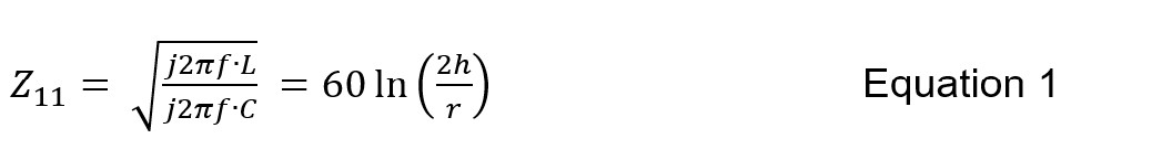
The surge impedance Z11 in Equation 1 has units of ohms. The double subscripts indicate it is the self surge impedance of conductor 1 with radius r1. If there is another conductor 2 nearby, then there will be a “mutual surge impedance” Z12 from Equation 2 that will equal Z21.
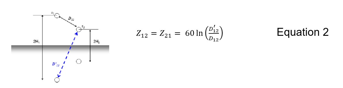
If a voltage impulse is applied to conductor 1, current of V1 / Z11 will flow. A fraction of this voltage, C2 V1 will appear on conductor 2, even if it is insulated and no current flows in it. A matrix of surge impedance values can be constructed from the conductor positions and the conductor radii. The calculations in Fig. 17 include the height of the conductors at the tower, and their average heights along the span, given by heights at the tower minus 2/3 of the sags.
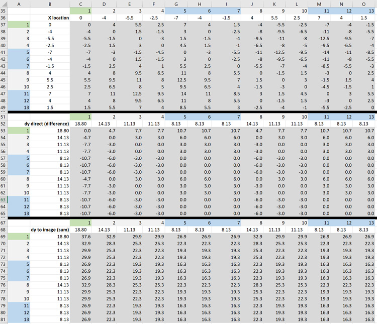
The everyday tensions of the transmission and distribution circuits are assumed to be the same, 20% of the rated tensile strength of the conductors. This is typical for transmission lines and the same tension is likely to be used for the distribution line conductors below, so that the sags match. The dimensions in Fig. 17 are used along with partial cell references such as C$36 and $B37 in cell C37 to make a calculation based on the dimensions in row 36 C-O and column B rows 37-49. The first matrix is the horizontal separation, the second matrix is the vertical separation for D12 and the third matrix in Fig. 18 is the vertical distance to the image conductor for D’12.
Once the distances between the conductors have been formed up, Equation 1 and Equation 2 are used to compute a surge impedance matrix as shown in Fig. 19.
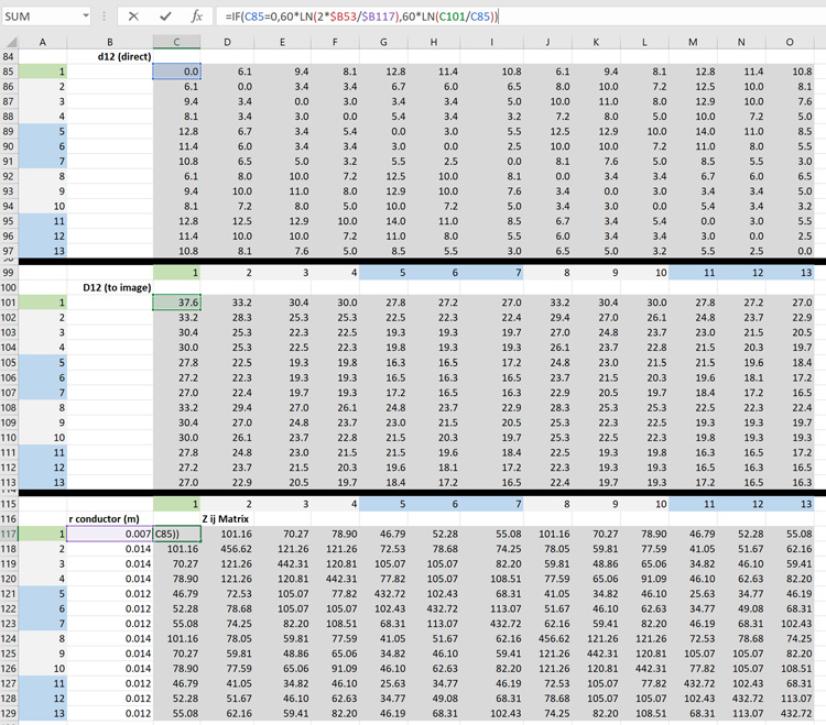
Microsoft Excel has built-in matrix functions: MMULT and MINVERSE. A search on-line can provide strategies for inverting complex matrices, but for lightning calculations these are not needed. The square [Zij] matrix in Fig. 19 can be multiplied by a vector of currents [Ii] to yield a vector of voltages [Vi]. The Excel help files eventually reveal that the way to see all the voltages from a matrix multiplication is to set up [Z], for example in cells C117-O129 in Fig. 19, then set the vector of currents [I] nearby in cells Q117-O129, then:
• Highlight all the cells where the voltage values will appear, perhaps S117:S129
• Type “ = MMULT(C117:O129,Q117:Q129) ” without the quotes
• Press F2, then press (all together at once) CTRL, Shift and Enter
This will place curly braces {=MMULT(C117:O129,Q117:Q129)} and all thirteen voltages will appear in the designated area.
The same process works with the MINVERSE function if you want to invert the impedance matrix and multiply it by a vector of voltages to obtain a vector of currents in each conductor. However, it is not correct to assume that the currents in driven phases will all be the same. More recent versions of Excel anticipate that users will want to see all calculation results from matrix operations.
Coupling Coefficients for Single OHGW
Fig. 20 implements the multiplication of a surge impedance matrix for the line in Fig. 17 by a vector of currents, with 1 A impressed into the OHGW (conductor 1, shaded green). The other twelve conductors are insulated and have no current. The voltage rise on the OHGW is, as expected, 515 V from its surge impedance Z11. What is more difficult to visualize is that voltages between 47 and 101 V appear on all the other conductors, because of their mutual surge impedance.
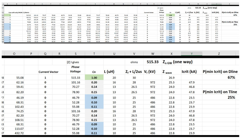
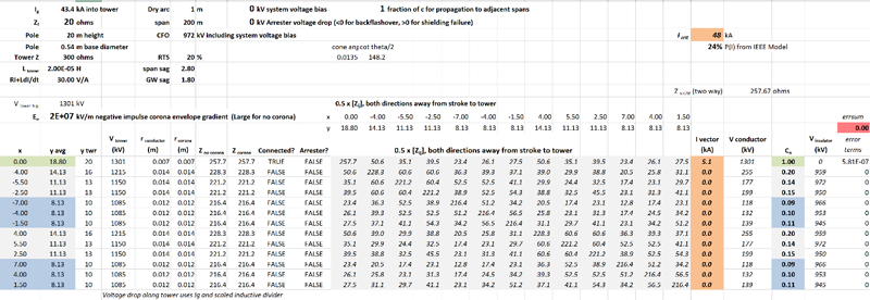
The coupling coefficients Cn highlighted in Fig. 20 are used in an implementation of the Fig. 13 Icrit calculation for each of the phases. The flashover voltage computed for the 115-kV insulator with 1 m dry arc distance, with 200 m span length, is 972 kV and the flashover voltage for the distribution circuit is half of that, 486 kV. The column labeled Zwave in Fig. 20 is the inverse of the denominator in Fig. 13. The critical currents for each phase in the next column are computed from the insulation strength, divided by Zwave, and corrected for coupling by dividing by (1-Cn).
The minimum critical current in this calculation, using Zf = 20 Ω, is 23.5 kA and the probability of exceeding this current is about 67%. Thus, two of every three lightning flashes will cause at least one flashover on a distribution circuit. The lowest critical currents on the transmission circuits are computed for conductors 3 and 9, which are the outermost phases. The probability of exceeding 46.8 kA is computed to be 25%. This is the performance that we would expect for a transmission line that had the same dimensions, but no distribution underbuild.
There is an important lesson in these results. The distribution line has poor lightning performance, even though it has overhead groundwire protection, because its 0.5-m insulation is relatively weak. The 115 kV line, with 1 m of insulation, would have an outage rate that is 2.7 times lower. This is offered as a reason why most transmission circuits are shielded, while most distribution circuits are not.
Coupling Coefficients for Arresters on All Distribution Insulators
It is inexpensive to purchase surge arresters for distribution systems. Most products today offer a strong track record of reliable electrical performance. Rather than fitting 1 m insulators to the distribution system phases, we consider protecting each 0.5 m insulator with its own surge arrester.
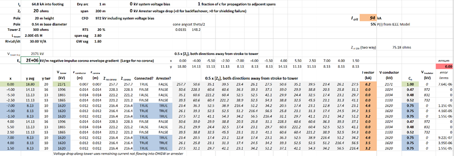
A quick estimate of the changes in coupling coefficient and increases in critical current can be made by altering the current vector in Fig. 20 to have unit currents in each protected phase. The spreadsheet elements in Fig. 17 to Fig. 20 were compacted into Fig. 21. The coupling coefficients and critical currents agree for single OHGW configuration. Then, the vector of currents is adjusted in Fig. 21 so that currents also flow into each of the six distribution system phase conductors.
Each surge impedance matrix value in Fig. 21 is exactly half of the values in Fig. 19. In the consolidation, the formulas implemented the fact that equal currents flow in two directions away from the tower into any OHGW or conductor that has been protected with an LSA. Also, voltages that appear on the bottom crossarm, highlighted in blue in Fig. 21, are lower than the voltage at tower top highlighted in green because the inductance from bottom crossarm to the ground is lower.
Fig. 21 shows that the value of Icrit for the transmission circuits increases from 48 to 94 kA when ideal arresters are fitted to all six phases of the two distribution circuits. This would give a 5x reduction in the lightning outage rate, based on the change in probability from 24% down to 5%. This compares favorably with most grounding improvement campaigns in terms of capital and maintenance costs as well as long-term effectiveness and thus forms an important transmission line rebuilding option.
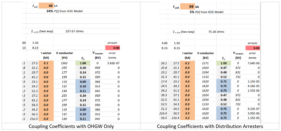
without (above, left) and with (below, right) LSA on distribution circuits.
Further Improvement in Coupling: Impulse Corona
Under ordinary operating conditions, high voltage engineers understand that high local electric fields can cause partial discharges such as corona. The corona may be benign – for example an ultraviolet signature at the end of a cotter key on an insulator cap. In some conditions, such as heavy rain, the corona may be intense, with distinctive audible noise as well as broadband electromagnetic radiation from the conductor-antenna gaps. The corona may be an indication of ongoing damage to insulators. Technologies of solar-blind ultraviolet cameras can sometimes distinguish a corona source. Generally, lines should be free of corona in clear, dry conditions and this makes UV cameras an important line inspection tool.
Under lightning surge conditions, corona switches from “enemy” to “friend”. The high voltages computed using the model in Fig. 13 cause envelopes of corona to form around towers and conductors. These have the following effects:
• Corona causes an increase in capacitance to ground. The CIGRE model (CIGRE WG 33.01, October1991 revised 2021) assigns a value of 0.0033 pF/kV/m to the excess of the applied voltage Um over the corona onset voltage of the conductor, Uci;
• The increased capacitance causes a reduction in parallel surge impedance Zn GW of any overhead groundwires and any arrester-protected phases that have voltage greater than Uci;
• The reduced surge impedance of conductors in corona causes an increase in coupling coefficients from the driven (OHGW or arrester protected distribution phase) to undriven (unprotected transmission phase) conductors;
• Corona (in the form of soil ionization) can reduce the footing impedance Zf for large currents;
• Corona effectively slows down the propagation speed to adjacent spans, and limits the amount of current that is shared among three or more spans of short length.
One of the most interesting differences between IEEE (IEEE, September 2008) (EPRI, 1982) and CIGRE (CIGRE WG 33.01, October1991 revised 2021) practice is the treatment of corona. The IEEE includes corona on the overhead wires with a simplified model, and ignores it when evaluating footing impedance, using the rationale that the currents required to make substantial soil ionization are too large to be relevant to the backflashover calculation. By contrast, CIGRE makes the corona effects on the OHGW difficult to model in electromagnetic transient programs, but their TB 63 (CIGRE WG 33.01, October1991 revised 2021) does include a simple model for soil ionization. Recently, both overhead wire corona models were criticized as inadequate (Rizk, Negative Impulse Ground Wire Corona Parameters for Backflash Evaluation of High Voltage Transmission Lines, August 2022) and an improved model was introduced.
The IEEE model assumes that there is a fixed voltage gradient at edge of the corona envelope, Eo. This was set to Eo =1500 kV/m for negative polarity in (EPRI, 1982). The corona radius Rc (m) is then given by:
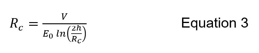
Where h is the average conductor height above ground (m) and V is the applied voltage. If Rc is less than the physical radius of the conductor, there is no corona and no change to the surge impedance matrix.
Equation 3 is “recursive” but converges rapidly. Any initial starting point – for example RC = 1 m – can be used. After 5 such calculations, each time using the fresh value of Rc, the final value is obtained. This is essentially a closed-form solution, and the function MAX(Rc, rconductor) will finalize the model so that low-current events do not cause corona but large-current events do.
The process in CIGRE TB63 (CIGRE WG 33.01, October1991 revised 2021) establishes a corona inception gradient Eci as:
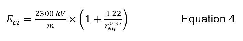
Where req is defined as the diameter of the conductor in cm. Streamer theory (Rizk, Negative Impulse Ground Wire Corona Parameters for Backflash Evaluation of High Voltage Transmission Lines, August 2022) leads to a similar estimate:
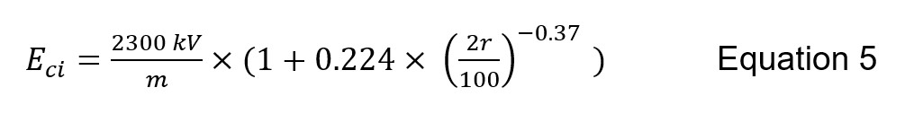
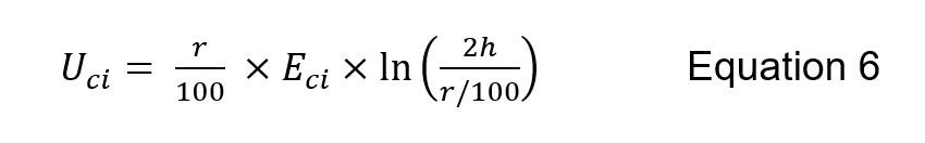
Where r is the conductor radius in cm. The impulse corona inception voltage Uci (kV) is computed using Eci (kV/m), the conductor radius r in cm (not req) and average height over ground h (m):
Conductor surface roughness factors, for example m = 0.7-0.9 in Peek calculations, apply for ac and dc operating conditions but not under impulse voltage stress.
In the CIGRE model (CIGRE WG 33.01, October1991 revised 2021), the rise in voltage above Uci adds extra capacitance to the natural value, Cn obtained from surge impedance Zo and travel time at the speed of light. A fixed value of 0.0033 pF/kV/m is valid for a conductor height of h = 25 m, but Rizk (Rizk, Negative Impulse Ground Wire Corona Parameters for Backflash Evaluation of High Voltage Transmission Lines, August 2022) found a strong variation with height, for example 0.0063 pF/kV/m for h = 10 m. This variation was modeled using two dimensionless ratios: Ccor/Cn and (Um – Uci)/Uci. Parameters a and b in their relation vary as a function of height h (m):

In all three cases, the corona envelope modifies only the capacitance term in the surge impedance, not the inductance. The effective surge impedance Zc under corona based on (Ccor/Cn) for Um > Uci is:
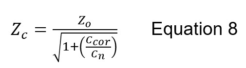
Where Zo = 60 ln (2h/(r/100)) (Ω) is the surge impedance when h is in m and r is in cm. All the corona models in Fig. 22 predict a reduced surge impedance with increasing voltage above Uci.
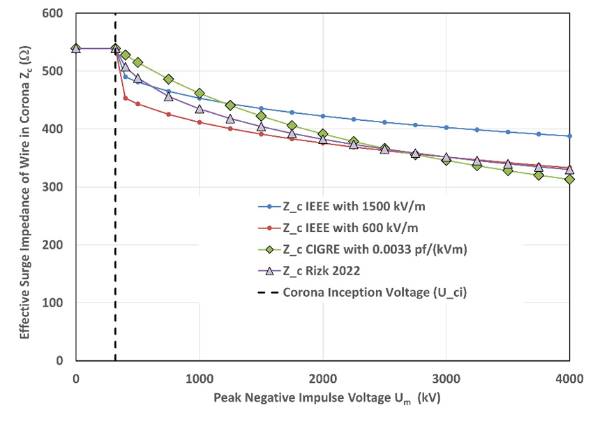
In the range of Um < 1000 kV, the traditional IEEE model with corona envelope gradient Eo =1500 kV/m in Equation 3 seems reasonable, but as Um increases, its values of Zc are too high. This could be “fixed” by reducing Eo, perhaps to a value of 600 kV/m, but this then causes problems for Um < 1000 kV. There is no single value of Eo in Equation 3 that matches the Rizk model well in all applications. Since the Rizk model in Equation 7 and Equation 8 is as easy to use as the IEEE / Anderson model, it is recommended for backflashover calculations moving forward.
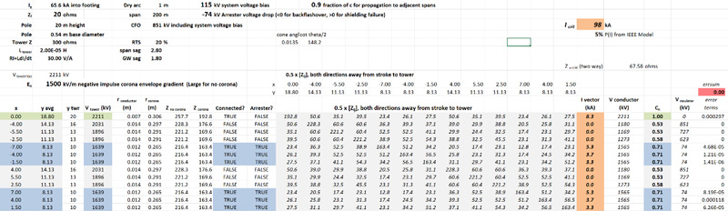
In (Chisholm W. A., Arrester Protection of Lower Voltage Circuits on Multi-Voltage Towers: Issues & Opportunities, October 20-23, 2019), the value of Eo = 1500 kV/m for negative polarity corona was used along with a footing impedance of 20 Ω and arresters on all six bottom phases. Figure 23 shows that the predicted critical current was 98 kA, with a 5% probability of exceedance.
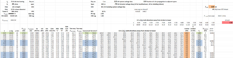
Thus, the improved model of impulse corona effects on surge impedance (Rizk, Negative Impulse Ground Wire Corona Parameters for Backflash Evaluation of High Voltage Transmission Lines, August 2022) and coupling is easy to implement and has enough of an influence on the results that it should be included in future backflashover analysis.
The situation for ionization of footings in soil remains less clear. Frequency dependence of soil resistivity offers the best explanation for good performance of transmission lines with high footing impedance. The effects of frequency-dependent resistivity have been verified in many practical field studies as described in the work of CIGRE Working Group C4.33. The Korsuncev ionization model (Chisholm & Janischewskyj, April 1989) used in (Rizk, Novel Solution to Back Flashovers on High Voltage Transmission Lines: The Embedded Ground Conductor, December 2022) suggests that a monopole foundation in the soil will start to ionize at a current well below the anticipated Icrit level, such that Zf for 30 kA may be less than half of the low-current values. However, it is difficult to support these calculations with testing, especially since high-resistivity soil may support a higher gradient of up to 1500 kV/m compared to 200-400 kV/m reported for low-resistivity soils.
Fully Insulated Crossarms
The concept of a 110 kV transmission line on fully insulated structure was put into service in 1933 (Ohio Brass Company, 1955).
providing 7300 kV CFO (+ 1.5/40) to ground and 1600 kV +CFO phase to phase (Ohio Brass Company, 1955).
This line delivered an outage rate of 0.7 per 100 km per year (Class B) mainly because it is in an area of low Ng.
The use of wood crossarms to supplement strings of ceramic discs is also common. The wood path offers benefits of increased impulse insulation, defined by the CFO-added method in (IEEE Power & Energy Society, Transmission and Distribution Committee, 2011 Jan 28). It also offers a degree of ac arc quenching, especially if an ac gradient < 10 kV/m can be respected (IEEE, September 2008). This is balanced by problems with splintering and splitting, as well as the possibility of pole fires initiated from insulator leakage currents.
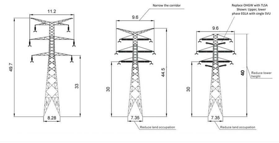
Recently several different types of composite insulated crossarm (CICA) have been described and applied to transmission rebuilding projects. The CICA in Figs. 26 and 27 stabilize the horizontal motion of the conductors, making the improved line compact. This allowed for reduced tower width as well as increased vertical clearance, which improved the line thermal rating.
The CICA in Fig. 27 provide 1841 mm of clearance from the conductor to the remaining tower steel. This dimension was substituted for the 1-m dry arc distance on the transmission circuits in Fig. 15. The critical currents and probabilities of being exceeded in Table 3 show that the CICA alone can achieve better lightning outage rate with Zf = 20 Ω than the as-built line with Zf of 10 Ω. Thus, CICAs provide an option to improve lightning performance and line thermal rating at the same time.
The last line of Table 3 shows that excellent backflashover performance can be achieved using CICA with 1.8 m clearance in combination with two underbuilt groundwires, modeled here as two of the 6 distribution phases fitted with surge arresters.
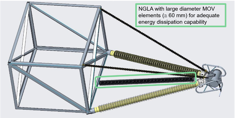
Recent developments to integrate TLSA into CICA have evaluated both EGLA and NGLA options. Successful integration could even lead to the elimination of OHGW, which would be replaced by heavy-duty arresters mounted as shown in Fig. 28.
Earthing
The final aspect to be considered when renovating overhead lines is the footing impedance. This plays two roles. Table 3 shows that the efficiency of backflashover protection depends to a large extent on the footing impedance Zf. In the background, however, is the insight from the 2-μs rise time in the simplified model. All the earthing that receives and dissipates lightning currents within 2 μs of the tower base will be useful. Any part of a grounding system that exceeds the “effective length” leff has limited benefit. The low-frequency resistance of local earthing systems, and inductive reactance of OHGW connections to adjacent structures, dominate the division of ac fault current and affect electrical safety calculations (CIGRE WG B2.56, 2017 07).
Recently, a series of papers (Grcev, Markovsi, & Todorovski, April 2023) evaluated a set of seven different counterpoise configurations to manage Zf. The configuration “GS5” is common in many countries, notably France and Brazil. Generally, the overall length l is increased in higher resistivity soil, up to the point where it achieves no further benefit under lightning surge conditions. Whether horizontal or vertical, a good estimate of leff is given by leff = (ρ tm)0.5 with resistivity ρ (Ωm) and ramp rise time tm (in our case 2 μs). The role of leff is shown in Fig. 30 for a case with ρ = 750 Ωm, tm = 2.5 μs and leff = 43 m. Once the counterpoise length exceeds 43 m, the impedance does not change from its asymptotic value of about 9.5 Ω.
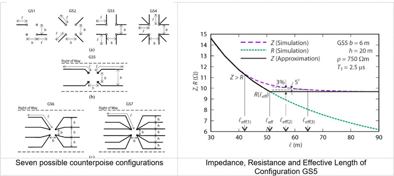
The work (Grcev, Markovsi, & Todorovski, April 2023) includes equations that describe the low-frequency resistance of each electrode in Fig. 30. A comparison was made from these individual expressions to the results from a general expression (Chisholm Formula) (Chisholm W. A., Evaluation of Simple Models for the Resistance of Solid and Wire-Frame Electrodes, November/December 2015), splitting the resistance into geometric and contact resistances.
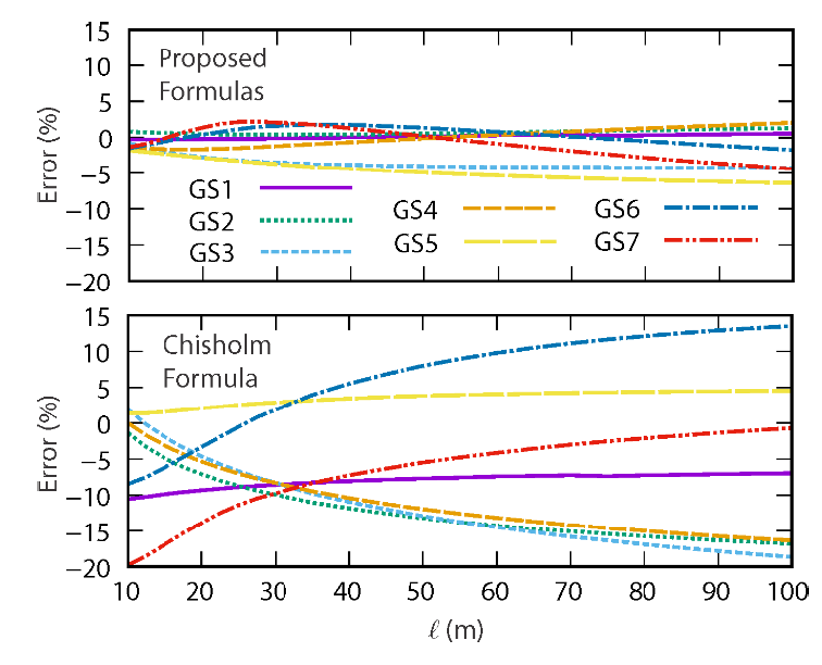
The error in the Chisholm formula relative to numerical reference calculations exceeds ±10% for some of the electrodes, while the individual formulas stay within ±6%. It is encouraging that the Chisholm formula in Equation 9 was found to be accurate for the common GS5 configuration and perhaps not surprising that it needs adjustment for long counterpoise with eight or twelve legs, not considered in the original development.
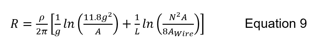
Where geometric radius g=√(rx2+ry2+rz2 ) where rx,y,z are the radial dimensions of the electrode (m) measured from its center, A is the overall surface area of the electrode (m2), L is the total length of wire (m) and wire surface Awire is L × 2π r for wire radius (m). To make the best use of the effective length model, some estimate of the soil resistivity is needed for every structure. This is an area of rapid progress in remote sensing, especially to provide the fraction of clay content in depth 0-2 m as well as estimates of depth to bedrock of the soil.
Conclusions
Despite a wide range of lightning activity, measured using ground flash density Ng, the lightning performance of a transmission line is expected to fall in a narrow security range, from Class C (<4 outages per 100 km per yr) of 69 kV lines up to Class A (< 0.5 outages per 100 km per yr) for UHV lines.
Transmission lines with a decade of service in 1955 tended to have span lengths of 180-250 m and often made use of wood components to achieve critical positive lightning impulse flashover strength of more than 1000 kV. Unshielded lines had poor normalized outage rates (corrected for thunder day) compared to shielded lines, with or without counterpoise. These lines are candidates for today’s rebuilding projects since they hold places on valuable rights-of-way.
The decades where transmission lines were rebuilt specifically to improve their lightning performance have passed. Now, other motivations such as damage repair or increased thermal rating are dominant. It is now the goal of the lightning protection engineer to ensure that these modifications also enhance, or at least do not degrade, the lightning and grounding performance.
Quantitative measures of Ng are available with uniform detection efficiency especially for regions within ±55° latitude. The increasing use of ‘total’ lightning detection systems introduces confusion by tabulating each ground termination point and each of the subsequent strokes. This greatly inflates the reported flash density but also takes it further away from the grouping that defined Ng for use in calculating lightning incidence to overhead lines: all flashes within 20 km and within 1 s.
Records of unshielded transmission line lightning performance can be evaluated using modern estimates of flash density to establish new flash incidence models that are not based on the traditional Ng.
Several lightning mitigation technologies, thought to be recent, had operating experience in 1955:
• Use of protector tubes, now “current limiting gaps”, to interrupt power follow current;
• Use of underbuilt groundwires (UBGW);
• Use of fully insulated (wood + porcelain) structures;
• Use of insulating (wood) crossarms in series with porcelain.
A case study applied non-gapped line arresters (NGLA) to a poorly shielded phase of a 115 kV line in 1997. After a series of problems, the line was restored to its original configuration by 2023.
The higher surge impedance of structures with improved visual aspect degrades the lightning backflashover performance.
A four-circuit mixed transmission / distribution line, evaluated previously for treatment with low-cost arresters across the distribution circuit insulators, was re-evaluated using an improved model of conductor corona. The new model (Rizk, Negative Impulse Ground Wire Corona Parameters for Backflash Evaluation of High Voltage Transmission Lines, August 2022) was easy to implement in Excel and predicted greater benefits from underbuilt groundwires and phases protected with arresters, compared to the widely used IEEE corona model (IEEE, September 2008).
Modern composite insulated crossarms (CICA) resolve problems with wood paths in series with insulation. They also stabilize the horizontal movement of phases (compaction) and raise the clearances (improved ampacity). Work to integrate TLSA into CICA is ongoing and promising.
Improved understanding of counterpoise for grounding leads to advice not to exceed its effective length, given by square root of resistivity (Ωm) and ramp rise time of 2 μs. Thus, leff in 200 Ωm soil is 20 m, and leff in 10,000 Ωm soil is 141 m. Since there is a large tower-to-tower variation in resistivity, each earthing treatment needs to be customized. This added test burden ensures that programs for improved earthing are not as effective as fitting of TLSA, UBGW and/or CICA in line rebuilding projects to improve or restore lightning performance to the desired security class.
[inline_ad_block]