Utility grids consist of large numbers of components and numerous connections that comprise a network supplying energy. While electric light and power supply started out as separate multi-client installations during the 1880s, by the 20th century, most electricity grids had become state-controlled and regarded as a public service offered at whatever cost required. These grids tended to be overdesigned, over-serviced and often deployed in only a national context. By the end of the century, however, energy came to be recognized as strategic and no longer at any cost since it was a significant component of production and needed to be controlled due to growing international competition. In addition to reliability, demand for cost-efficiency became a priority.

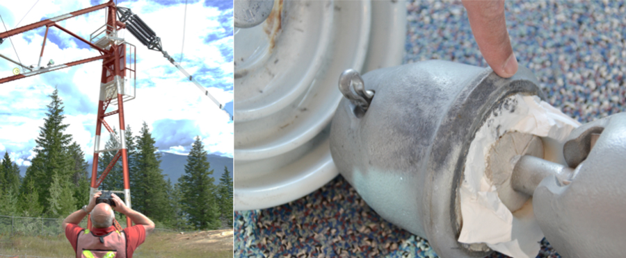
Components and connections in any grid and must meet the requirements of power supply. Yet most grid assets wear due to mechanisms driven by temperature, electromagnetic field, mechanical forces, vandalism and ambient conditions such as salt fog and acidity. As such preventive as well as corrective maintenance actions are required. Ultimately, replacement becomes necessary. Cost, human resources, materials as well as planned outages make up the efforts and the risks for power utilities. Not undertaking such efforts creates added risk and maintenance strategies therefore require proper consideration.

This edited past contribution to INMR by Robert Ross, Reliability & Asset Management Dept. of the Institute of Science & Development and Chair of Performance of HV Energy Systems at Delft University of Technology in the Netherlands, reviewED asset management as well as the Corrective, Period-Based, Condition-Based and Risk-Based maintenance styles and where these are most applicable. Redundancy plays an important role in grids to safeguard security of supply. With the tendency to postpone replacement and to harvest as much operational life of assets as possible, redundancy is put to the limits. This article therefore also devotes attention to quality loss of redundancy whenever service life of assets is prolonged. One important conclusion is that, even in the absence of failures, an unwanted situation may build up where redundancy is no longer effective.

---

Listen to Online Lecture on Asset Replacement Strategies in Ageing Grids

Background

Need for cross-border electricity trade in various areas of the globe grew as a way to secure energy supply and cost-efficiency. Internationalization was one of the consequences of the drive towards secure energy supply, keeping energy affordable, protecting the environment, reducing climate change and improving electricity grids. For example, in the case of Europe, energy policy has been summarized as “sustainable, secure and affordable”. This policy had far-reaching consequences. Traditional electricity grids were organized as a chain consisting of power plants interconnected to a high voltage transmission network as well as a distribution network. Electricity sales to industry and other end-users also belonged to this utility service. By the end of the 20th century, however, this traditional utility chain was effectively broken up and electricity production and sales were privatized.

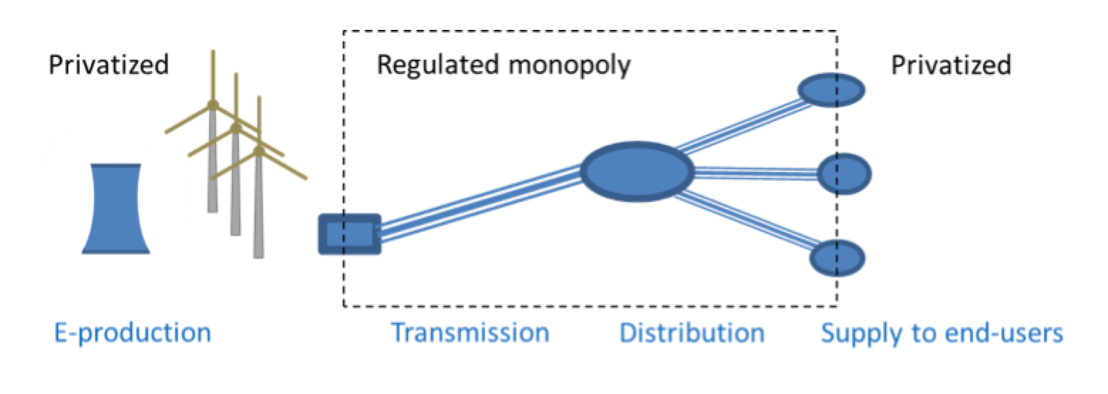
Grids are so capital intensive and have such impact on spatial planning that neither investments nor added right-of-ways were available to build competitive infrastructure in parallel. As such, there is usually only one electricity grid shared by all providers. Network utilities therefore kept a monopoly on electricity transmission and distribution. Nevertheless, in pursuit of cost efficiency and affordability, many countries installed Regulators to supervise and set market prices and also quality standards. This assured that grid owners/operators could not unreasonably drive up prices for their transmission and distribution services. In this way, while utilities kept physical monopolies, they were compared to worldwide best practice and faced penalties if underperforming either by poor power quality or excessive expenses.

Precise tasks and formulations might differ somewhat by country but the responsibilities of Distribution System Operators (DSOs) and Transmission Operators (TSOs) typically comprise maintaining an electricity network and also providing connections between producers and consumers. Furthermore, TSOs have the task of maintaining a balance between supply and demand for electrical power. In this context, asset management by power utilities aims to provide a resilient, secure and cost-efficient infrastructure. This leads to solutions that differ from those employed during most of the 20th century when technical quality of reliable electrical energy supply faced far fewer constraints on financial and workforce resources (as usual with most public services). In addition to Corrective Maintenance (CM) and Period-Based Maintenance (PBM), new maintenance styles such Condition-Based Maintenance (CBM) and Risk-Based Maintenance (RBM) were developed, supported by tools such as diagnostics, condition monitoring, health index and risk index. CBM focuses on functionality of grid components. RBM also takes into account the consequences of dysfunction, measured in terms of business values that can include safety, power quality, security of supply, etc. However, CBM and RBM are not necessarily always more feasible or more cost-efficient than conventional styles such as CM and PBM.

Aspects of Maintenance

Physical grid components are the tangible assets that together shape network infrastructure. Asset Management (AM) is the collective term for structured decision-making and execution of plans so as to reach some optimized balance between performance, efforts and risk with utilization of these assets. An AM system is therefore an organized set of systematic and coordinated activities with the goal of staying in control. Various standards have been developed for common practice in AM, including PAS 55 and ISO 55000.

One important aspect of asset management is selecting the most suitable maintenance style(s). Maintenance is defined here as comprising the activities of inspection, servicing and replacement. The longer components can be utilized, the more value is retrieved. At the same time, the more costly the maintenance, the less profitable is such delay in investments. Moreover, if functionality is jeopardized and failures occur, with possibly significant consequences, business values could be severely violated. Liability and mitigation costs as well as damage to reputation could rise disproportionally and waste all the benefits from prolonging the operating life of ageing assets.

Given this, how can asset management best contribute to sustainable, secure and affordable energy? Below is a review of various maintenance and configuration optimization dilemmas. First, basic aspects of maintenance and replacement are discussed to set the context and offer definitions. Next, this information is applied to diagnosable assets. Finally the role of redundancy is studied.

Maintenance Activities & Styles

Maintenance of the grid and its components can be defined in various ways, and, for the purposes of this discussion, subdivided into three main classes of activity:

• Inspection

Activities or monitoring to assess the functioning and condition of assets;

• Servicing

Activities to restore or enhance functioning and condition of assets, usually aiming to prolong their lifetime;

• Replacement

Removing an asset and installing a usually new asset.

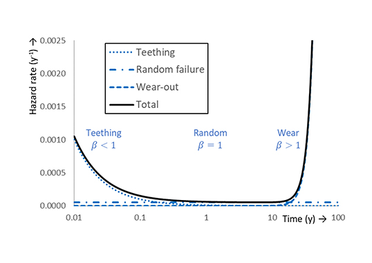
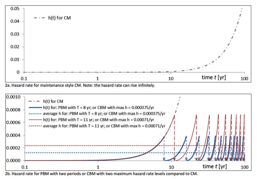
The above maintenance styles can be applied to each of the three activity classes. Fig. 2 shows how maintenance styles respond to so-called hazard rate, h, that is a measure of the likelihood that a working asset will fail in the near future. A description of these styles is as follows:

• Corrective Maintenance (CM)

Actions taken to restore required functionality after whatever malfunction has been noted, usually meaning repair (i.e. servicing) or replacement. One advantage is that the full lifetime of the asset is realized but a disadvantage is that failure can occur suddenly and without warning. Moreover, flexibility is required to respond adequately to potentially hazardous additional failure events. Emergencies of this sort are usually far more costly to resolve than are planned actions.

• Period-Based Maintenance (PBM)

Preventive action (i.e. inspection, servicing, replacement) that is planned based on some variable, e.g. number of running hours, number of switching actions, etc., and not based solely on passage of time. The advantage of PBM is that it allows efficient planning of resources and efforts and also prevents failures. A disadvantage, however, is that planning is based mainly on the weakest performing assets in a batch and therefore not optimized for cost efficiency. Excess maintenance and higher replacement costs tend to be linked with PBM but the gain is remaining in control.

• Condition-Based Maintenance (CBM)

Preventive action based on the perceived functionality/condition of an asset. This requires diagnostic methods to assess condition as well as knowledge rules to properly interpret diagnostic results in terms of remaining life before breakdown or possibly required reduction in load. The advantage of CBM is that maintenance is tuned to the individual asset. A disadvantage is that much flexibility is required since the utility has to always be in a position to respond appropriately to whatever events take place. How much time is left for mitigation depends on type of the relevant process, on availability of adequate diagnostic tools, on adequacy of knowledge rules for interpreting results and on when evaluation is being made.

• Risk-Based Maintenance (RBM)

Preventive action based first on perceived functionality/condition of assets and second on extent to which a failure event or malfunction could violate key business values such as safety, liability, financial impact, etc.. RBM is not necessarily more cost efficient than CBM but aims at better overall performance in terms of such corporate values, which may or may not be easy to monetize.

Though technology and information required could differ between styles, it cannot be said that one style is always superior or more efficient than another. Rather, whichever style is most suitable depends more on purpose, on balance between operational versus capital expenses (i.e. investment) and also on circumstances. For example, pressurized oil cables can be checked periodically for oil pressure (i.e. PBM inspections) and the oil replenished if necessary (i.e. CM/CBM servicing). Similarly, polyethylene-insulated cables are typically never inspected but instead repaired in the event of failure (i.e. CM servicing) or, if forensic analysis so indicates, replaced (i.e. CBM/RBM). Finally, utilities might employ periodic replacement schemes, e.g. replacing cable after 40 or 50 years (i.e. PBM replacement). While this sacrifices part of their residual operating lifetime, it may save on costs linked to emergency repair. Moreover, PBM allows for easier planning. In practice, utilities may have reasons to apply a mix of all these styles.

Reliability, Availability, Redundancy & Reparability

Reliability, R, is related to likelihood that a system fulfills its function. Assets are supposed to work properly at time of commisioning while their operational life ends either with failure or removal for other reasons. Inspection and servicing makes it possible to extend operational life by employing PBM or CBM maintenance styles. R is equal to 1 minus probability of failure, F:

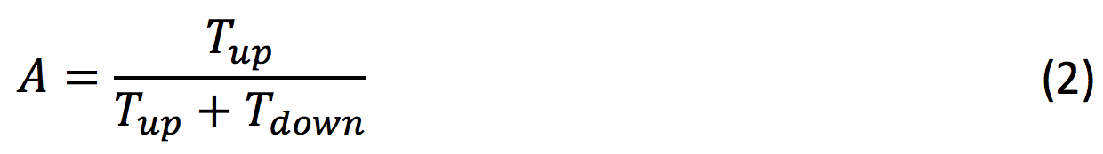
Some systems, however, can be repaired after failure. This may not hold true for individual components but usually applies for a circuit, connection or grid repaired by replacing the faulted component. Reparable systems balance between a ‘working’ and a ‘failed’ state, i.e. there are periods that the system functions and times when it has failed and is under repair. Availability, A, is defined as the ratio of the time, T_up, from getting available to function until failure and the total time T (which is the sum of T_up and the downtime, T_down, after failure, until the assets return to operation):

One certainty is that any event that can occur will indeed someday happen, however unexpected. In most power grids, this certainty is usually taken into account using two distinct measures. In addition to the above maintenance styles, these are:

• Redundancy

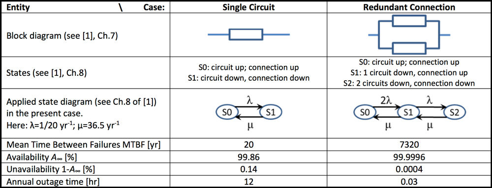
Installing a connection as a double circuit (or higher redundancy), as in Table 1, prevents failure in a single circuit to down the connection. Of course, the system is less or even no longer redundant after a failure. Moreover, failure in the second circuit, before repair of the first, downs the entire connection.

• Rapid Repair

If a system is reparable after failure, quicker restoration of functionality (i.e. higher correction or repair rate) reduces risk of a simultaneous circuit malfunction and increases availability of the grid.

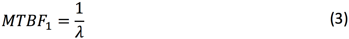
Combining redundancy and rapid repair/replacement is common practice in strategic infrastructures. The effect of this approach can be calculated with so-called Markov chains. While it is beyond the current scope to discuss such complex mathematics, a typical result is summarized. First, consider a connection without redundancy, i.e. a single circuit. Assume that a failure rate, λ, and a repair rate, μ, apply. Mean time between failures (MTBF₁) of this circuit is then:

 

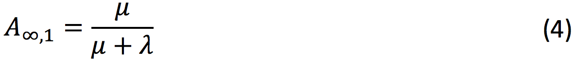
In the long run, availability A_∞,1 of the circuit is:

Now, consider the case of a connection consisting of a double circuit. Assume that each circuit has failure rate, λ, repair rate, μ, (single repair only) and that each circuit is able to carry the full load. In this case, mean time between failures (MTBF₂), i.e. between events leading to a simultaneous outage of both circuits, is: (note that usually μ >> λ)

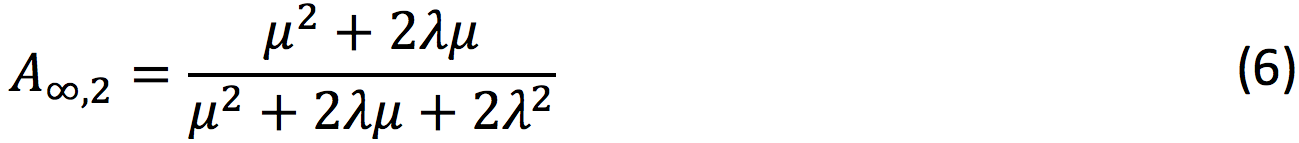
In the long run, availability A_∞,2 of this connection is:

To make it more practical and for comparison purposes, assume that the circuit would fail once every 20 years (λ=1/20 yr^-1) and that a typical repair would bring the asset back into service in 10 days (μ = 0.1 d^-1 = 36.5 yr^-1). Table 1 compares the MTBF and A_∞ of the single circuit as well as of the redundant connection with two parallel circuits. Results show that the MTBF of the redundant connection is 366 times that of the single circuit. In other words, unavailability, 1-A_∞, of the single circuit is much greater than for the redundant connection. The single circuit provides average availability of more than 99%. In common terms, any percentage greater than 99% may be regarded satisfactory but for a strategic service such as power supply this is generally insufficient. Indeed, given a grid with possibly thousands of connections and if each connection is out of service for half a day per year (i.e. the 12 hr mentioned in Table 1), numerous corrective actions will be required. At the same time, there is considerable social and economic disruption. It is therefore not uncommon to require MTBFs to fall in the range of thousands of years, e.g. to exceed 5000 yr.

To avoid misunderstanding, the meaning of MTBF > 4000 yrs. is not that such assets are expected to have an operational lifetime τ > 4000 yrs. but rather that an asset in that condition would fail only once every 4000 yrs. at most. In other words, if there are 4000 assets in that condition, then it is expected that not more than one will fail in a single year. The fact that the asset can age and have a much higher failure probability after e.g. 40 years means that its MTBF shrinks during the wear-out phase. The challenge for utilities then is to find some optimum in asset management. A high degree of redundancy can be effective in building a reliable grid but is also costly if this means doubling or even tripling the investment needed for the single non-redundant solution. Most Regulators require utilities to apply a certain level of redundancy (particularly for heavier connections) because of the strategic importance of electricity supply. Moreover, achieving rapid repair depends on factors such as logistics, standardization of components and techniques, strategic storage of spares, having multiple suppliers of services and components, existence of maintenance contracts, etc.

System and/or Circuit Reliability & Availability

How should utility performance and efficiency be evaluated when it comes to replacement and what is the basis for replacement strategies? For example, is it reliability and availability of the usually redundant system or rather of each circuit? The primary task of a TSO and DSO is to transmit and distribute electrical power. However, as discussed, Regulators also set boundary conditions, e.g. the EU policy mandates sustainable, secure and affordable energy. Redundancy allows having a failure without interrupting power supply (assuming the reserve does not fail during the repair period). This seems to imply that maintenance style CM is preferable. In principle, maybe, but considering that business values other than solely uninterrupted service also apply, redundancy should not be overly associated with CM. For example, if an asset such as a cable termination or transformer fails, this can be a violent event involving explosion or fire that endangers safety and could also cause significant collateral damage to other assets at the substation. Therefore, redundancy should never be an excuse for careless operation.

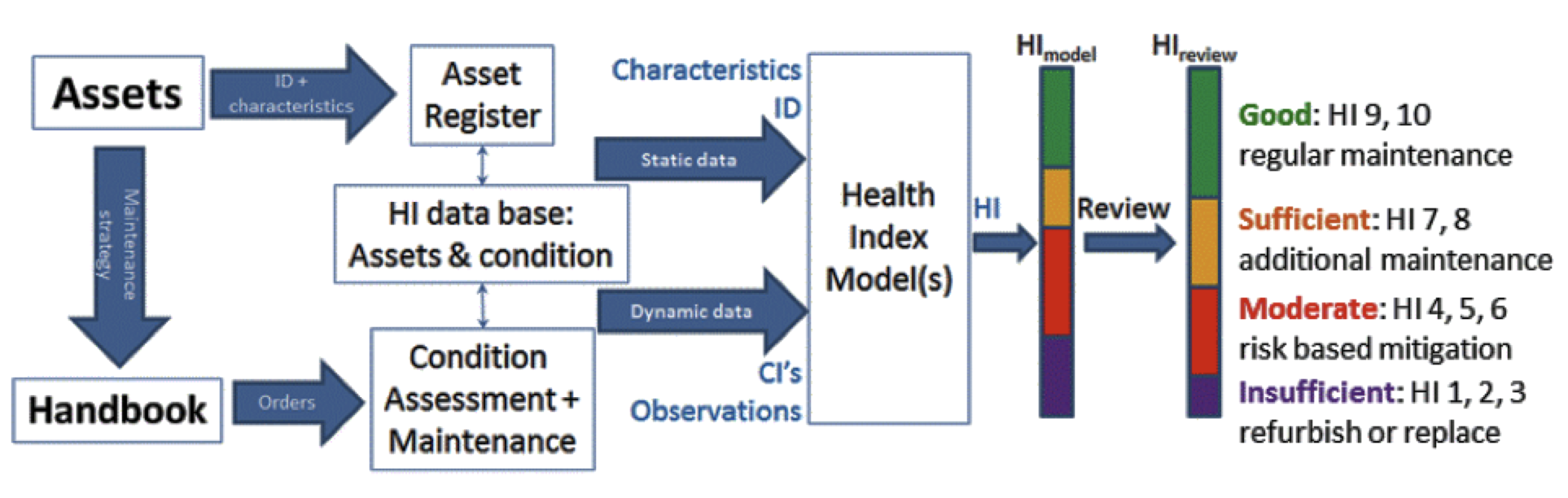
Given this and in order to best keep track and rank priorities, many utilities these days employ Health Index methods (see Fig. 3). Health Index (HI) is a score for the health (i.e. condition) of an asset and also indicates the perceived hazard rate or remaining life of that asset. In the case of CBM, this is used as the basis for decisions on maintenance actions, including replacement. HI is generally applied to single assets. It would make sense to upgrade this methodology to a Combined HI (CHI) at the level of circuits, connections, substations, sub-grids etc. in order to best prioritize and coordinate maintenance. One way to achieve this is to link HI to hazard rate since this can be calculated for various system configurations and repair actions. This way, not only assets but also reliability and availability of circuits can be evaluated and scored.

In an RBM approach, the risks to utility business values lead to prioritizing maintenance actions. The probability of a failure event occurring is multiplied by the impact that such an event can have. This maintenance style provides a strategy to take into account threat to safety and other hazards. For evaluation of risks, so-called risk matrices (or in the continuous variant: the risk plane) lead to a Risk Index. The risk that a redundant system can go down is part of the evaluation with the aspect of security of supply. The following elaborate examples to compare such strategies in practice. Firstly, situations will be studied where the condition may be diagnosed (whether economically efficient or not). Secondly, redundancy is studied when hardly any information on condition is available. In the latter case, the situation is analyzed by assumed distributions.

Diagnosable Assets

If the condition of an asset can be assessed with sufficient confidence, all three maintenance styles – CM, PBM and CBM – are in principle feasible. If the impact of failure is known as well, then RBM also becomes feasible. Which of these maintenance styles is deemed most appropriate then depends on cost and possibilities of preventive maintenance when comparing CM and PBM. Both maintenance styles treat all assets the same. CM lets all assets run to failure and takes advantage of their full operational life but the impact of unforeseen failure could be high and flexibility is required to respond adequately to failures. Since failures are part of this asset management style, redundancy is commonly employed to warrant continuous power supply. Part of the gain by employing the full asset life could be cancelled by increased investments in redundancy. The need for redundancy may be higher for CM than for PBM since PBM sacrifices asset life in order to prevent unplanned outage. Emergency situations should occur less frequently with PBM than with CM.

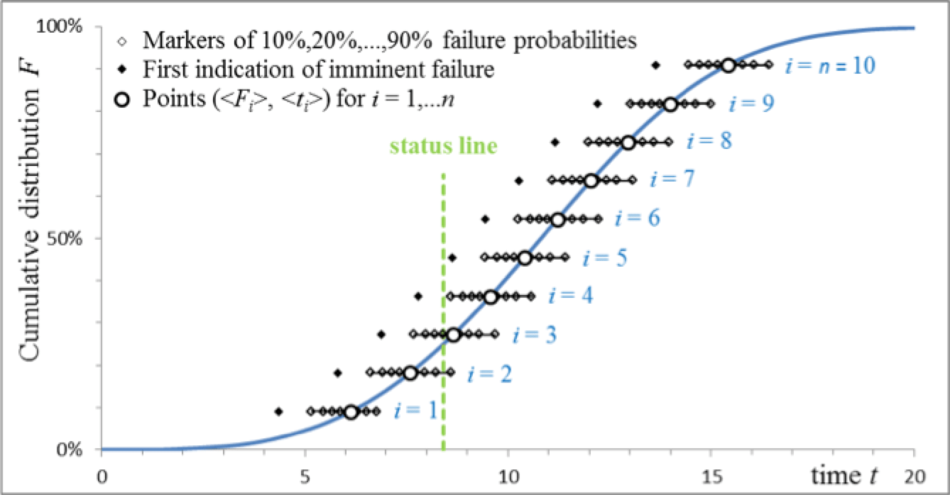
When comparing CBM and PBM, the largest gain of CBM lies in utilizing information on the individual assets. Fig. 4 below shows the distribution of failure times of a group of 10 assets. It is assumed that each failure is preceded by a detectable signal that indicates imminent failure of that asset. Failure likelihood per asset is shown by the percentage markers as a representation of failure time probability after the first indication of imminent failure. For example, if the green status line in Fig. 4 defines the moment of evaluation, assets i=1-4 have already signalled that failure is imminent (i=1, 2 may have already failed), while assets i>5 have not yet given any alert. This is essential in CBM, which allows to timely plan and mitigate the situation with assets i=1-4. By contrast, if PBM is applied, all assets would be replaced or serviced well before the first fails (otherwise the management style becomes CM). PBM might therefore dictate replacement at the moment cumulative distribution reaches e.g. 1% level at t=3 (arbitrary units). CBM would allow operation on average until about t=11 (arbitrary units). So, on average, lifetime in this case would triple that achieved with PBM. CBM requires adequate diagnostics and adequate expert rules to judge need for mitigation.

CBM techniques and rules often require more advanced technology than CM or PBM and can also be more costly. Evaluating whether or not such investments are worthwhile is a fundamental part of asset management.

Not all assets allow for sufficient diagnostics and the condition of some assets cannot easily be diagnosed at all. The choice is then between CM and PBM. Applying redundancy is one established method to prevent interruption of power supply. But with an ageing population of assets, the growing fear is that CM and CBM will lead to large numbers of assets that require attention simultaneously. The question also arises as to how effective redundancy is in the case of older assets.

Evaluation of Redundancy Without Data on Failure or Diagnostics

Over the past years, quite a number of assets have approached or even surpassed their original planned lifetimes. Often, a replacement wave was predicted that did not in fact materialize. Indeed, many assets have been operated within their original specifications and live longer than anticipated at time of commissioning. However, replacement of assets such as cables and transformers require long lead times that hinder adequate and timely mitigation in cases where replacement becomes urgent. So, is there nothing to worry about or is it possible that, despite absence of failures, a replacement wave is about to emerge? And, if so, what strategies are recommended?

By way of warning, there have been assets that did not meet their planned lifetimes. One particular danger occurs since redundant circuits are usually installed at the same time as part of a single project. The idea of redundancy is that the good cable, for example, can fully take over when a parallel cable fails. However, if both cables are of the same age and design, while wear out becomes significant, do the circuits still provide sound redundancy? Or could the situation arise where one bad component becomes the spare for a failed one? And, can such a situation grow without any indications or warnings? How fast can a grid condition deteriorate unnoticed?

If the condition of an asset cannot be assessed and, while no failures have yet taken place the operational life of the asset is about to exceed that planned or is already beyond that, the question becomes: how effective is redundancy? In the following, a case is described where no failures took place as yet and adequate diagnostics are not available. The goal is to verify whether or not it makes sense statistically that a redundant circuit with no recent failures should nevertheless still be regarded as suspect. The following steps are made:

a. Define the case of a cable connection and define a repair rate based on utility practice;
b. Set criteria for required mitigation based on asset condition levels in terms of perceived hazard rates;
c. Set boundary conditions for the ruling statistical distribution and its failure rate based on international experience;
d. Evaluate whether the hazard rate of the redundant circuit indeed indicates need for replacement.

Case History

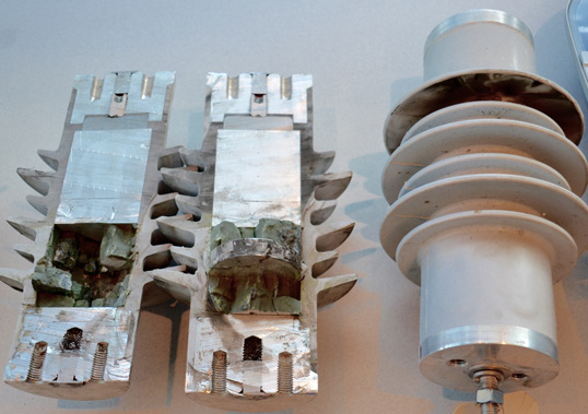
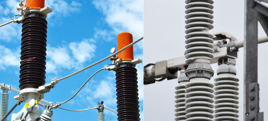
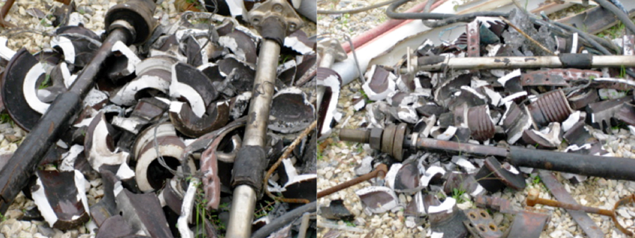
The example considered below involves a redundant 150 kV cable connection consisting of two parallel self-contained oil filled (SCOF) cables each with a length of 1.25 km. The cables feature 2 terminations and 3 joints. Therefore, each circuit consists of 3 single phase cables, 6 terminations and 9 joints. At the moment of evaluation, the connection has been in service for 56 yrs. but does not show any signs of degradation or occurrence of faults. In fact, some parts of the cable circuit may be even older but such information is not fully traceable. For this case, therefore, an age of 56 yrs is adopted. The circuit is believed to have been operated below its rated load throughout its service life. However, power demand is growing and the connection may soon be operated at rated load. Is absence of failures sufficient to believe that this connection is sound?

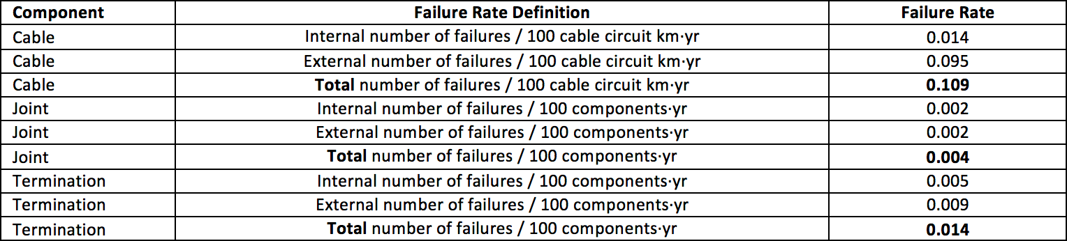
Each circuit can fail due to various incidents such as a wearing joint or termination, degraded cable insulation or failure due to a random process unrelated to any degradation process (e.g. lightning strike). The circuit survives if it survives all failure mechanisms. In system reliability theory this is a series system. As a consequence, circuit hazard rate is the sum of all respective process hazard rates. Cigré B1 regularly evaluates worldwide experience with cables and, in order to adoptan objective reference, average failure rate over a lifetime of 40 years is taken from the work of WG B1.10 (shown in Table 2 below). It should be noted that WG B1.57 is currently drafting an update in which failure rates will most likely differ from these and the outcome of the present analysis is then also likely to differ with the new data. Still, the methodology remains the same and TB 379 is used here to define reasonable hazard rate.

The failure rate λ_av of a single circuit is therefore:

Taking into account circuit kilometers and number of components, the result is:

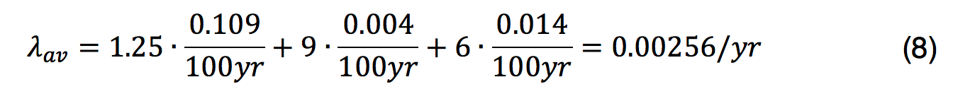This is taken as the average failure rate of the cable circuit over 40 yrs. (which was the design lifetime at the time the cable was produced). Given that the cable is wearing, failure rate will be low at the start but increase over the years. A similar development to that shown in Fig. 2a can then be expected. Normally, there is some steady hazard rate, λ_cnst, not related to wear and resulting increased hazard rate, and with an average, λ_wear,av. Total average hazard rate λ_av is:

 

What values these hazard rate have will depend on individual utility and also on the country where it operates. TB 379 suggests that the majority of failures are due to external causes, though not necessarily unrelated to wear. Here, it is assumed that λ_cnst=1.042∙10^-3 yr^-1. Average hazard rate for wear over 40 yrs. is λ_wear,av = 1.521 • 10^-3 yr^-1. Note that momentary wear, λ_wear(t), is an increasing function of time and after 40 yrs. is expected to possibly be significantly larger than average, λ_wear,av.

Criteria for Replacement

Criteria for action are not standardized. RBM describes a product of occurrence frequency (i.e. rate of occurrence or failure rate) and a measure of impact. Some utilities translate all impacts into financial damage (i.e. monetizing) while others employ an impact gravity scale. At this stage, risk scaling is a matter of culture and preference. Generally, with any given impact, risk index varies with failure rate. In the present case, for the situation where both circuits fail and blackout the entire 150 kV connection, Table 3 shows the boundaries. Note that Risk Index comes with its own color scheme which is not necessarily the same as that for Health Index. Other risks may or may not give rise to a higher risk index due to a higher occurrence rate and/or impact. The hazard rate, h, applies to the connection and is defined as the inverse MTBF.

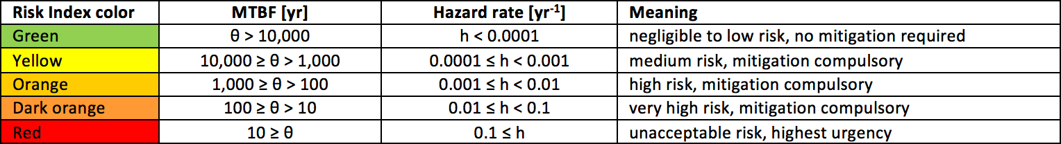
Table 3 can then used to evaluate need to replace. If the MTBF, θ, of the redundant connection drops below 10,000 years, then corrective action is compulsory and replacement justified. This MTBF, as explained above, does not depend only on circuit failure rate, λ, but also on repair rate, μ, as shown in equations (5) and (6). A repair rate of μ =1/26 yr^-1 is assumed for this type of cable.

Ruling Distribution

In the present case, no failure data are available which is at the core of any such case. To evaluate whether the situation can be suspect, a reasonable worst case scenario is therefore designed. The present boundary conditions are:

• No failures during the past 40 years;
• Random failures are possible with a constant hazard rate, λ_cnst, over time;
• Wear is expected to develop and corresponding hazard rate, λ_wear(t), can be expected to increase over time;
• Momentary circuit hazard rate, h_circ(t), can be calculated by summing the hazard rates, λ_cnst and λ_wear(t);
• Average h_av of the momentary hazard rate, h_circ(t), over the period 0-40 yrs. is assumed equal to the Cigré average hazard rate, λ_av , according to [7], Table 2 above and Eq. (9).

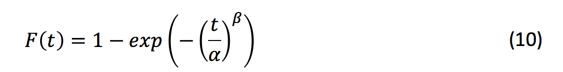
Cables fail usually at their weakest point and are examples of weakest link in chain cases. Therefore, Weibull distributions generally apply. The two parameter Weibull distribution has a scale parameter, α, and a shape parameter, β. A Weibull distribution is employed in the following and cumulative failure distribution, F(t), is defined as:

The corresponding hazard rate of the Weibull distribution is defined as:

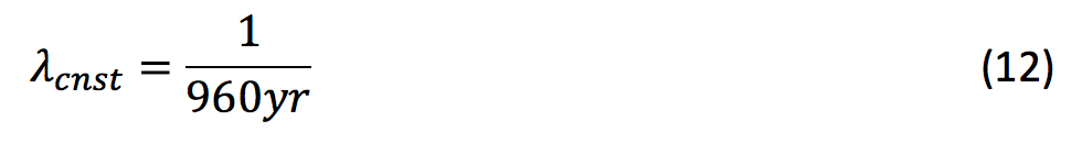
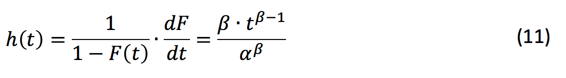If β=1, then hazard rate becomes a constant equal to α^-1. The constant hazard rate, λ_cnst=1.042 • 10^‑3 yr^‑1, mentioned in Eq. (9), can therefore be described by a Weibull distribution with α_cnst=(λ_cnst)^‑1 = 960 yr and β_cnst=1:

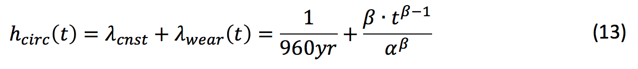
The challenge now is to define a suitable Weibull distribution for the wear-out mechanism that matches the boundary conditions above. Here, the purpose is to demonstrate how to study the likelihood that a suspect situation arises unnoticed. For the sake of simplicity, a Weibull based hazard rate h_circ(t) is designed that is not refined to discriminate the separate contributions of joints, terminations and the cable but rather just fits a single wear-out process (note: it is not difficult to design a refined multi-parameter-set model). The idea is to define a momentary circuit hazard rate, h_circ(t), from which the connection MTBF, θ_conn, can be estimated. This momentary hazard rate is the sum of the mentioned Weibull based λ_cnst and λ_wear(t):

The parameters, α, and shape parameter, β, must now be chosen such that the mean of h_circ(t) over the period 0-40 yrs. equals the average λ_av=0.00256 yr^-1 mentioned in Eq. (8). Table 4 shows a selection of parameter sets (α,β) with resulting h_circ.av over the period 0 to 40 yrs. These sets were chosen by first setting a value for β in a range that is common for paper degradation and then fine tuning α and β such that h_circ.av ≈ λ_av=0.00256 yr^-1.

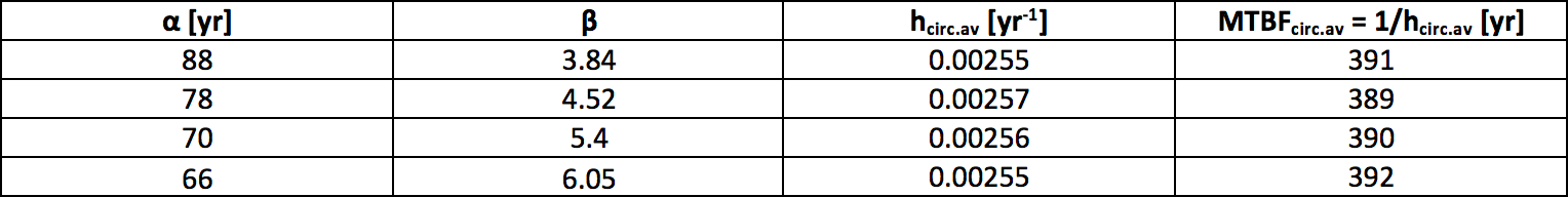
Lacking experimental data it is not possible to assess the actual ruling failure distribution. However the parameter sets in Table 4 all fulfill the boundary condition that the average hazard rate over the first 40 yr about equals 0.00256 yr^-1. It is explored in the following whether such sets can induce a situation that should be mitigated.

Hazard Rate & HI for Overdue Circuits

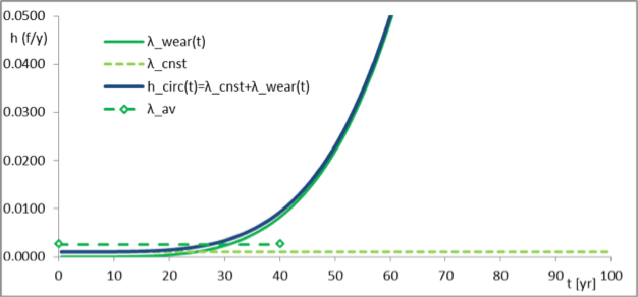
First the results for set (α,β) = (70 yrs.) are presented, after which an overview is given of other results. Fig. 5 shows how circuit hazard rate develops over time. The figure shows hazard rates for random failure λ_cnst, wear-out failure λ_wear(t) and h_circ(t) as sum of both. Adopted average hazard rate level, λ_av, over the first 40 years is also shown. Already, before the 40 years have passed h_circ(t) lifts off but with an MTBF of 390 yr it is highly possible that the cable did not yet fail. The moment of evaluation is t = 56 yrs and then the circuit hazard rate h_circ = 0.0358 yr^-1. With circuit hazard rate, λ = h_circ, and the repair rate, μ, the MTBF can be calculated with Eq. (5), which appears θ(56yr) = 10,189 yrs. This is very close to the limit θ = 10,000 yrs. below which mitigation is compulsory according to Table 3. In fact, 1 year later at t = 57 yrs. this limit is exceeded, as shown in Table 5. This is an example of a case where it is not necessarily noticed that the connection has degraded to a level where mitigation becomes compulsory. Does this indicate that the situation out of control? No, the risk is medium and while higher than allowable, not yet high. Nevertheless, good asset management practice requires following up the risk before it becomes high.

Quantitatively, if the (α, β) = (70 yrs.) set applies and if there are 1/h_circ = 28 circuits in similar condition, then one of those circuits will likely fail per year. If there are 10,189 connections in a similar condition, then one of those connection per year will likely blackout. Rather than regarding such failures as an incident, it may be realized that a much larger group may exist and that this is a structural development. The case description also mentioned that the cable may see higher load in the future. This means that temperature will rise and paper insulation will be increased. In addition to the present wear-out effect, higher load will mean that the α parameter will be reduced and ageing speeds up. The present analysis does not take that into account but in a more comprehensive analysis this is recommended.

The third and fourth columns of Table 5 below show the circuit hazard rate and its inverse at the moment of evaluation (i.e. t 56 yrs). The fifth and sixth column show the connection hazard rate for black-out of the connection and the inverse hazard rate. The seventh and the eigth columns show the year in which the connection hazard rate exceeds the limit 0.0001 yr^‑1 respectively 0.001 yr^‑1. These limits are the border between green and yellow respectively and between yellow and orange (c.f. Table 3).

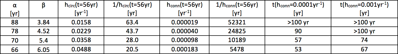
Table 5 shows the results for all parameter sets listed in Table 4. It shows that the parameter choice has large impact and which would apply is not known since data is lacking. Each reasonable assumption can be considered. If data from comparable cable circuits would be available, this would help. The most important message is, however, that even redundant circuits that show no failures as yet, can still require mitigation. The background lies in the quality of redundancy. A step further is to investigate the effectiveness of redundancy. It may be noted from Eq. (3) and (5) that the MTBF of a circuit inversely declines with circuit hazard rate, but recalling μ >> λ in general, MTBF of a connection declines with the square of the circuit hazard rate. This means that redundancy itself deteriorates faster than do the circuit mean-times-between-failures.

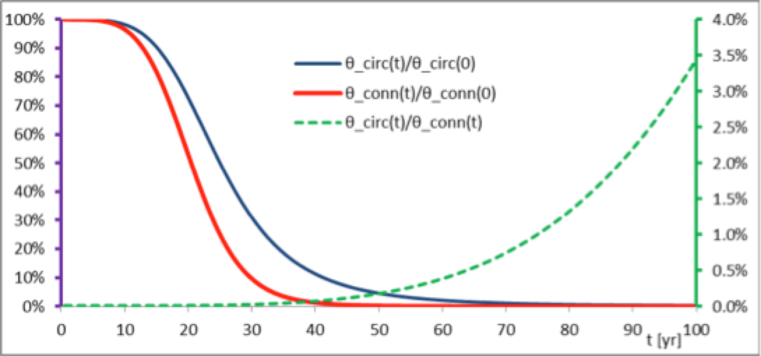
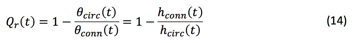
Fig. 6 also compares the connection and circuit MTBF θ (right-hand vertical axis scale). It underlines the decreasing quality of redundancy. Furthermore, this ratio may be used to define a quality of redundancy Q_r as 1 minus the ratio:

Circuit hazard rates are already a factor roughly 10 larger than the average hazard rate over the first 40 years. It is the decay in redundancy that is worrisome. Table 3 indicates that mitigation is already compulsory or soon will be. The solution can be replacement of one or both cables, which sacrifices cable operational life. Another strategy is to install a new, third parallel cable in the connection that changes the configuration and upgrades redundancy. The new situation can be analyzed by the Markov chain method. A third circuit requires a bay at the substations on both sides of the connection.

Summary

This article discusses the background of the transition to modern asset management. The Corrective, Period-Based, Condition-Based and Risk-Based maintenance styles are explained, along with the circumstances where these are most applicable. Particular attention is paid to the importance and role of redundancy. An estimation method is elaborated to evaluate situations, even if failure data are not available. Enhancement of the load in the future would further accelerate ageing. It is shown that, with prolonged deployment of circuits, the possibility exists that the connection must be mitigated. However, lack of failure data may just not give reason to study the case and reach the conclusion that mitigation is indeed necessary. A promising strategy to deal with ageing connections is to upgrade them with a third parallel cable, if the substation allows.

References:
[1] R. Ross, Reliability Analysis for Asset Management of Electric Power Grids, Hoboken, NJ: Wiley-IEEE Press|, 2019, pp. 4-20.
[2] British Standard Institution, “Asset management, Vol. Part 1: Specification for the optimized management of physical assets,” British Standard Institution, London, 2008.
[3] International Standards Organization, “ISO 55000: Asset Management – Overview, principles and terminology,” International Standards Organization, Geneva, CH, 2014.
[4] International Standards Organization, “ISO 55001: Asset management – Requirements,” International Standards Organization, Geneva, CH, 2014.
[5] International Standards Organization, “Asset Management – Guidelines on the Application,” International Standards Organization, Geneva, CH, 2014.
[6] R. Ross, “Health Index methodologies for decision-making on asset maintenance and replacement,” in Cigré 2017 Colloquium of Study Committees A3, B4 & D1, Winnipeg, Canada, 2017.
[7] Cigré WG B1.10, “TB379 Update of Service Experience of HV Underground and Submarine Cable Systems,” Cigré, Paris, 2009.