Distribution system engineers sometimes take advantage of existing transmission right-of-way to route their medium voltage (MV) circuits when standards show there is adequate vertical clearance to high voltage (HV) transmission circuits above. Often, the lightning performance of the HV circuit improves, while the trip-out rate of the MV circuit is disappointing.
In this edited past contribution to INMR, Dr. William Chisholm explained that line surge arresters offer an opportunity to retain the benefits of improved electromagnetic coupling of lightning to the HV circuit above while mitigating induced and backflashover overvoltages on the MV circuit below. With appropriate selection, arresters on the lower circuit can also mitigate cross-system contact faults
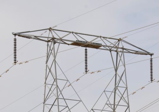
Fig. 1 shows a visually appealing arrangement of “delta” transmission circuits and “horizontal” distribution circuits, with 1-2-3 conductors balanced on each side.
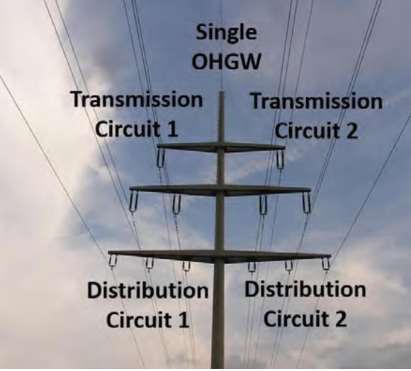
Lightning protection for this line is provided by a single overhead groundwire (OHGW), mounted at the top of the pole. Each steel pole is grounded but soil resistivity varies considerably from tower to tower so each pole will have a different value of footing resistance. The lightning performance of a structure with four circuits, arranged as per Fig. 1, will be considered. Assume the 115 kV transmission circuits have 1.0 m insulators and the 50 kV distribution circuits have the minimum recommended dry arc distance of 0.5 m. This line configuration will be used to visualize the concept of electromagnetic surge impedance coupling. Depending on the distance from the single OHGW, each phase will take up a voltage wave that is a faithful but reduced amplitude copy of what appears on the tower top. The voltage stress on each insulator is the difference between the local tower voltage rise and this ‘coupled’ voltage.
The insulation strength of the distribution circuits is so low that, for most lightning surges, some or all six bottom phases will flash over to ground. Each flashover will introduce a new path for lightning that changes the coupling. The strength of the coupling is expressed as a set of ‘coupling factors’, Cn, with individual values for each of the n conductors – twelve in Fig. 1.
A series of calculations will be made to establish an important parameter in the ‘backflashover rate’ that establishes the lightning outage rate of most lines. This is the ‘critical current’ Icrit that causes the voltage on one of the line insulators to slightly exceed its lightning impulse strength, resulting in a line-to-ground fault that follows and sustains the flashover arc.
A rough estimate of Icrit¬ can be obtained by dividing the insulator critical flashover voltage by the footing impedance, measured at the base of the stricken tower. There are a number of adjustments, each described in Standards for:
• The volt-time curve for impulse flashover: often a calculation is done for time to flashover in the range of 1 to 3 microseconds, and the evaluation time depends on span length;
• The surge impedance coupling from those OHGW, faulted and arrester-protected conductors that carry a fraction of the lightning surge current away in each direction from tower top;
• The additional voltage rise associated with fast-rising current flow in the inductance of the thin monopole structure;
• The variability of soil resistivity and footing impedance from structure to structure;
• The effects of corona, which absorbs energy from the lightning and reduces stress on the insulators;
• The effects of line voltage, as one phase will always have an instantaneous voltage that adds to the stress;
• The effects of line surge arresters on the distribution circuit of Fig. 1 that convert protected phases to extra groundwires and thus provide some benefits even to the unprotected transmission phases above
An initial calculation will compare results using a fixed value of footing resistance at each tower, incorporating a volt-time curve, surge impedance coupling and tower inductance. The computed value of Icrit, and the probability of exceeding it, will then be compared to a composite result based on a realistic log-normal distribution of soil resistivity that changes from tower to tower. The effects of impulse corona on Icrit will be demonstrated for the transmission circuit, with and without the distribution underbuild to show the improvement in coupling. At the assumed transmission and distribution system voltage levels (115 kV and 50 kV), power system voltage bias is not as important, but it does reduce Icrit slightly, increasing the backflashover rate by a factor of about 20%, independent of footing impedance. The surge impedance matrix is used to estimate the currents that will flow through each surge arrester placed in parallel with distribution system insulators. Based on these currents, the voltage drops across the arresters can be subtracted from the voltages on protected phases to re-assess the voltages that will appear on unprotected transmission phases.

Simplified Modeling of Backflashover Process in Excel
Selecting Appropriate Platform for Modeling Calculations
The 1982 version of the EPRI Red Book Ch, 12 introduced a step-by-step process for calculating the lightning performance of a transmission line. This algorithm was modified by IEEE and implemented in a series of computer programming languages: FORTRAN, BASIC, C, Visual Basic for Applications and Python as a series of FLASH programs. Hileman provided a similar set of BASIC programs to implement the CIGRE Technical Brochure 63 approach to estimating lightning performance. The BASIC version of the FLASH program in IEEE Standard 1243TM has recently been criticized by the IEEE Standards Association because it does not run directly in Windows 10 or other modern operating systems. The ability to execute these legacy programs is now managed using emulators, but it has been suggested that executable programs like FLASH should be withdrawn from future standards.
EPRI has faced a similar dilemma. It developed a series of “Applets”, based on the Java language, to support its revisions of lightning and grounding resources in the period 2005-2010. It was hoped that these would remain independent of operating systems and would execute successfully in any future web browser. Unfortunately, source code for EPRI applets is hidden to ensure program integrity and security and most have now been abandoned because they do not execute at all.
There remains a need to illustrate technical and statistical concepts mathematically. Microsoft ExcelTM seems to be the lowest common denominator used for this purpose. It provides adequate methods for matrix manipulation, iteration and statistical simulation to evaluate the changes in lightning performance that would be expected when distribution circuits are added below transmission circuits as in Fig. 1.
Backflashover Model Based on Fixed Ramp Time of 2 μs
It turns out that the original choice of a linear ramp wave with zero to peak time of 2 microseconds (2 μs) remains an excellent choice for evaluating the overvoltage that appears across insulators under lightning surge conditions. Measured downward negative first return strokes generally have a concave front that reaches its maximum derivative Smax, dI/dt just at the peak of the current wave. The equivalent ramp front time, extrapolating back from peak at the rate of Smax to zero current, seems to increase slowly in the range of 1.8 to 2.5 μs, depending on peak current magnitude. Fig. 2 fixes the zero-to-100% rise time of 2 μs and uses it to convert tower inductance to voltage rise, using the model DV = L dI/dt = LI/(2 ms). The voltage rise at tower top is the sum of footing voltage rise Zf ×I and L dI/dt. The voltage rise at intermediate positions along the tower is established by the current flow and the inductance from that point to the ground. This is often scaled linearly if the tower has a cone shape, like a steel monopole, with constant surge impedance viewed from the apex.
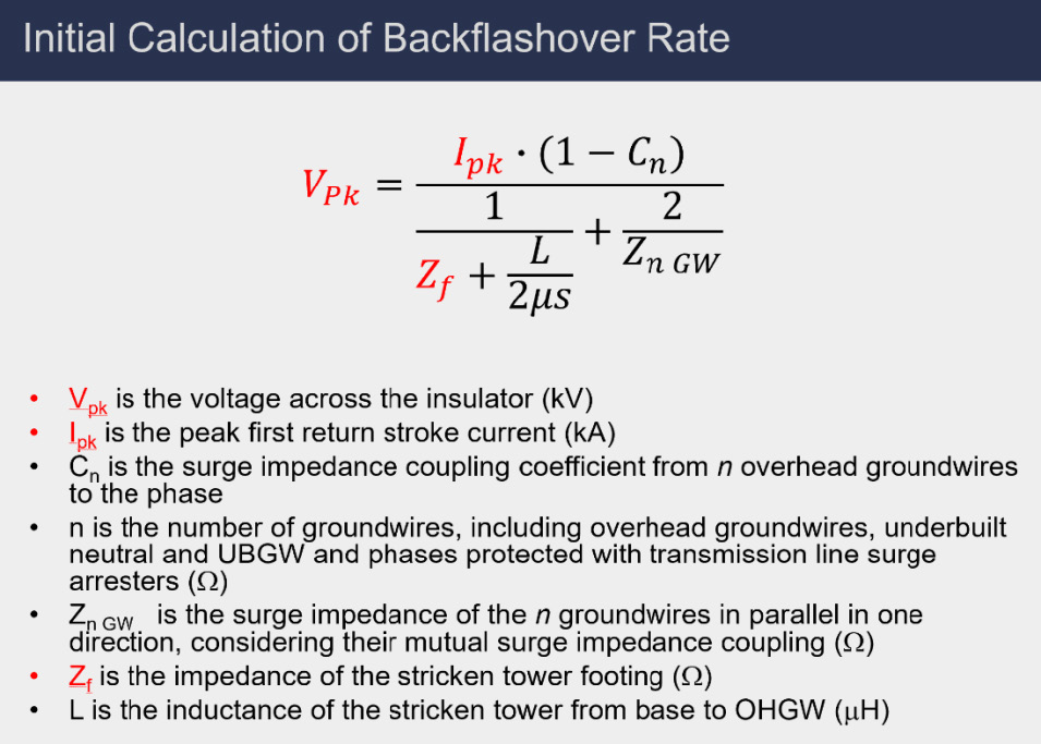
Backflashover calculations are normally carried out with the first negative return stroke parameters, because these have the largest values of Ipk that tend to give the highest levels of Vpk using Fig. 2. There is no single value for Ipk – instead, it is described by a log-normal statistical distribution, with median 31 kA and standard deviation of ln(Ipk) between 0.48 and 0.66.
Impedance of the stricken tower footing Zf depends on the size and shape of the buried portion of the tower. For a monopole, such as Fig. 1, depth of burial is commonly estimated as at least 10% of the pole length, plus 0.6 m. Pole heights and burial depths are relatively constant along a line section. However, the resistivity of the soil r (units of ohm meters or Wm) also has a log-normal distribution. The log standard deviation of resistivity, based on 300-m distance between sites, has been found to be in the range of 0.9 for regions in the USA and Portugal. This means that the distribution of Vpk, computed using the process in Fig. 2, is the product of two, very wide statistical distributions, meaning that failure is always an option, and we are engineering instead to a desired failure rate specification, such as one tripout per 100 km of circuit km per year.
Backflashover Model with Log-Normal Distribution of Footing Impedance
The Excel RAND() and LOGNORM.INV functions were used in Fig. 3 to illustrate how pole-to-pole differences in soil resistivity affect the lightning performance calculation.
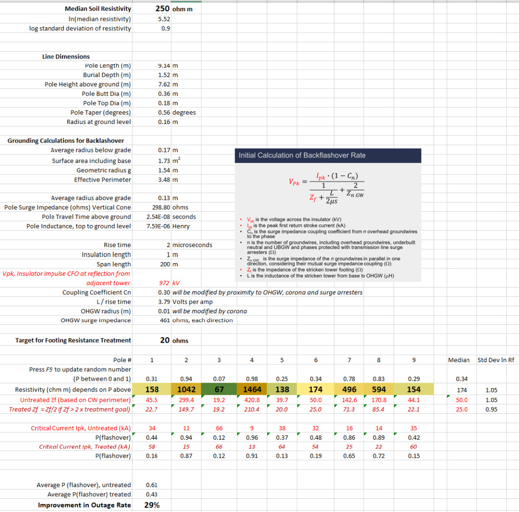
Nine poles are modeled. Each is given a random number RAND() between zero and 1. This probability is then used as an argument in the LOGNORM.INV(probability, mean, stdev) function. A median soil resistivity is found in the first row of 250 Ωm. This is converted to the mean of the log-normal distribution with LN(20) = 5.52. The log standard deviation value is fixed at 0.9. The nine colored cells in Fig. 3 then provide resistivity estimates that vary from tower to tower, with minimum of 67 Ωm and maximum of 1464 Ωm in this simulation run. Each time the F9 key is pressed, new probability values appear in each cell, and these update the rest of the calculations.
The model relating tower footing impedance Zf to resistivity r is simple but accurate. The geometric radius of the part of the pole buried in soil is computed to be g = 1.54 m, based mainly on the burial depth of 1.52 m. The surface area of this slightly tapered cylinder is A =1.73 m2. The expression Zf = r/(2pg) ln (11.8 g2/A) is inverted to give an “effective perimeter”, the equivalent hemisphere, of P=3.48 m. This is used in each case to convert resistivity to Zf using Zf = r / P.
The pole inductance L is computed from the surge impedance and travel time at the speed of light. Thus, the 299 W surge impedance times travel time of 0.254 ms gives an inductance L = tZ = 7.6 mH. When this is divided by 2 ms ramp time, the voltage rise associated with the pole becomes ΔV =7.6 μH / 2 μs = 3.8 Volts per Amp.
Rather than computing the insulator voltage Vpk for a random set of Ipk values, the calculation in Fig. 3 manipulates the expression in Fig. 2 to provide the ‘critical current’ based on a calculated value of insulator flashover strength. A volt-time curve for strings of ceramic insulators is used and the evaluation time is taken to be the point at which the voltage wave becomes non-standard – which is the time that it takes for current to make the back-and-forth trip to the adjacent two towers.
Backflashover Model with Log-Normal Distribution of Resistivity & Remediation Plan
The log-normal model of resistivity in Fig. 3 can be used to show the effects of a grounding remediation plan. Often, faced with poor lightning performance, asset managers will set in motion a project to improve the grounding resistance on a line. In a non-optimal approach, the same improvement, such as additional driven rods or buried radial counterpoise, will be installed at every tower. A better approach would set a target impedance value, for example 20 W in Fig. 3. Any structure with Zf > 20 W would be treated. If Zf is found to be in the range of 20 to 40 W, it is often practical to install enough new ground electrodes, within 60 m of the pole, to meet the target. However, for high-resistivity cases, the best that can be achieved is often a factor-of-two reduction. Thus, for example, at Pole 9, the initial value of Zf = 44.1 W is reduced to 22.1 W, making a significant reduction in the probability of flashover from 42% to 15%. However, at Pole 8, the reduction from 171 W to 85 W only reduces the probability of flashover from 89% to 72%. With a typical log-normal distribution of resistivity, the targeted grounding campaign would treat eight of nine poles and achieve a 30% improvement in lightning outage rate.
Backflashover Model with Arresters
Surge arresters, placed across the insulators, will limit the local overvoltage as they pass a fraction of current into the protected phase conductors. This has the desirable feature of increasing n, the number of groundwires, in Fig. 2. It will also affect the coupling coefficient, which was fixed at Cn=0.3 in Fig. 3 to focus on the role of log-normally distributed soil resistivity. There is always a question about who pays, and who benefits, when making a capital investment. When considering surge arresters on the distribution circuits in Fig. 1, a transmission engineer may be unsympathetic. There will be flashovers to the distribution circuits, bringing their phases in parallel with the OHGW, even if arresters have not been fitted. However, by understanding the relatively poor return on investment associated with grounding improvements, and the well-controlled improvements achieved by making the same investment in medium-voltage arresters, some equitable cost-sharing may be achieved.
Modeling of Electromagnetic Coupling on Four-Circuit Line in Excel: Surge Impedance Coupling Matrix
Most of the simplified programs for computing lightning performance have some limitations with regard to the number of circuits and groundwires. While there is only a single central OHGW in Fig. 1 applying LSA to the bottom six conductors will bring them into the surge impedance coupling circuit. This will be illustrated first with a linear model. Then, the effects of impulse corona on the surge impedance and coupling matrix will be explored. Finally, the effect of line voltage and voltage drops across the arresters will be evaluated.
Mini-Tutorial: Self & Mutual Surge Impedance Matrix
Impedance of a conductor over ground at power frequency is a complex number but as the frequency f increases from 50-60 Hz to over 100 kHz, the series resistance term becomes negligible compared to inductive reactance. The surge impedance of a wire, based on inductance L and capacitance C per unit length, converges to a scalar value:
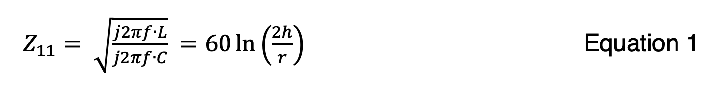 The surge impedance Z11 in Equation 1 has units of ohms. The double subscripts indicate it is the self-surge impedance of conductor 1 with radius r1. If there is another conductor 2 nearby, then there will be a ‘mutual surge impedance’ Z12 from Equation 2 that will equal Z21.
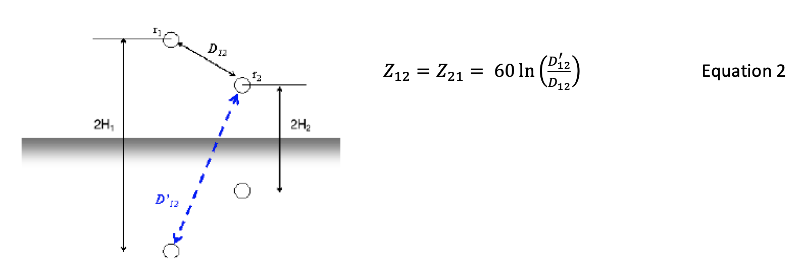 If a voltage impulse is applied to conductor 1, current of V1 / Z11 will flow. A fraction of this voltage, C2 V1 will appear on conductor 2, even if it is insulated and no current flows in it. A matrix of surge impedance values can be constructed from the conductor positions and the conductor radii. The calculations in Fig. 4 include the height of the conductors at the tower, and their average heights along the span, given by heights at the tower minus 2/3 of the sags.
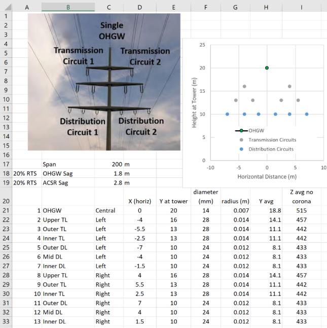
The everyday tensions of the transmission and distribution circuits are assumed to be the same, 20% of the rated tensile strength of the conductors. This is typical for transmission lines and the same tension is likely to be used for the distribution line conductors below, so that the sags match. The dimensions in Fig. 4 are used along with partial cell references such as C$36 and $B37 in cell C37 to make a calculation based on the dimensions in row 36 C-O and column B rows 37-49. The first matrix is the horizontal separation, the second matrix is the vertical separation for D12 and the third matrix in Fig. 5 is the vertical distance to the image conductor for D’12
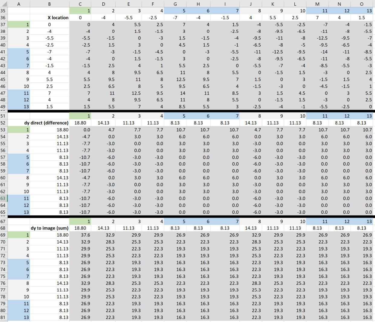
Once the distances between the conductors have been formed up, Equation 1 and Equation 2 are used to compute a surge impedance matrix as shown in Fig. 6.

Microsoft Excel has built-in matrix functions: MMULT and MINVERSE. A search on-line can provide strategies for inverting complex matrices, but for lightning calculations these are not needed. The square [Zij] matrix in Fig. 6 can be multiplied by a vector of currents [Ii] to yield a vector of voltages [Vi]. The Excel help files eventually reveal that the way to see all the voltages from a matrix multiplication is to set up [Z], for example in cells C117-O129, then set the vector of currents [I] nearby in cells Q117-O129, then:
• Highlight all the cells where the voltage values will appear, perhaps S117:S129
• Type “ = MMULT(C117:O129,Q117:Q129) ” without the quotes
• Press F2, then press (all together at once) CTRL, Shift and Enter
This will place curly braces {=MMULT(C117:O129,Q117:Q129)} and all thirteen voltages will appear in the designated area.
The same process works with the MINVERSE function if you want to invert the impedance matrix and multiply it by a vector of voltages to obtain a vector of currents in each conductor. However, it is not correct to assume that the currents in driven phases will all be the same.
Coupling Coefficients for Single OHGW
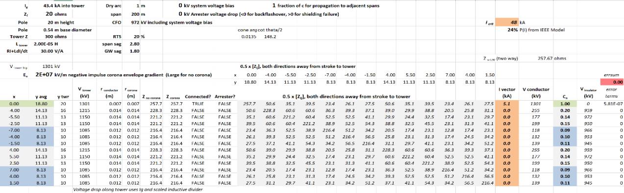
Fig. 7 implements the multiplication of a surge impedance matrix for the line in Fig. 4 by a vector of currents, with 1 A impressed into the OHGW (conductor 1, shaded green). The other twelve conductors are insulated, and have no current. The voltage rise on the OHGW is, as expected, 515 V from its surge impedance Z11. What is more difficult to visualize is that voltages between 47 and 101 V appear on all the other conductors, because of their mutual surge impedance.
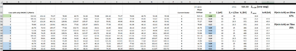
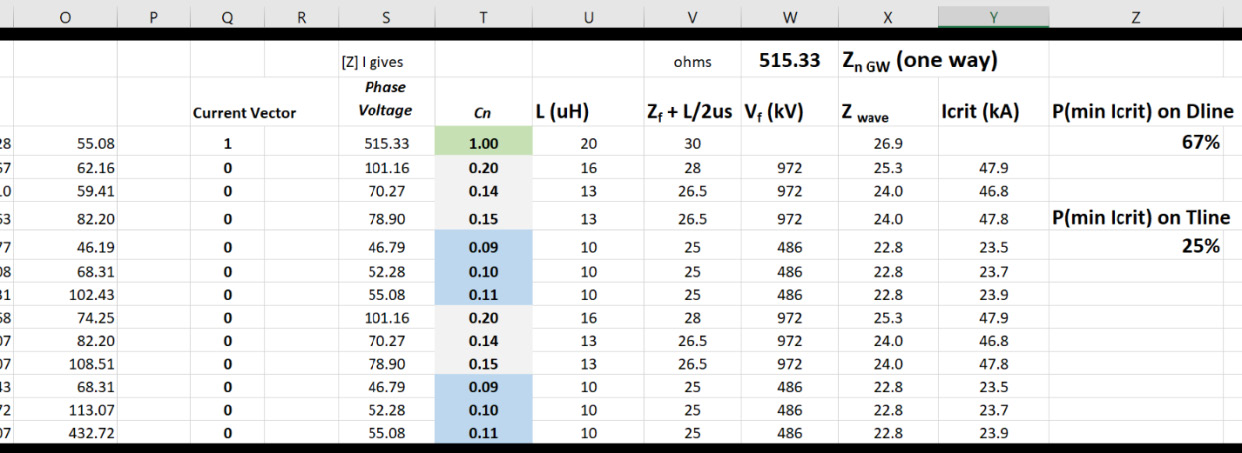
The coupling coefficients Cn are used in an implementation of the Fig. 2 calculation for each of the phases. The flashover voltage computed for the 115-kV insulator with 1 m dry arc distance, with 200 m span length, is 972 kV and the flashover voltage for the distribution circuit is half of that, 486 kV. The column labeled Zwave in Fig. 7 is the inverse of the denominator in Fig. 2. The critical currents for each phase in the next column are computed from the insulation strength, divided by Zwave, and corrected for coupling by dividing by (1-Cn).
The minimum critical current in this calculation, using Zf = 20 W, is 23.5 kA and the probability of exceeding this current is about 67%. Thus, two of every three lightning flashes will cause at least one flashover on a distribution circuit. The lowest critical currents on the transmission circuits are computed for conductors 3 and 9, which are the outermost phases. The probability of exceeding 46.8 kA is computed to be 25%. This is the performance that we would expect for a transmission line that had the same dimensions, but no distribution underbuild.
There is an important lesson in these results. The distribution line has poor lightning performance even though it has overhead groundwire protection, because its 0.5-m insulation is relatively weak. The 115 kV line, with 1 m of insulation, would have an outage rate that is 2.7 times lower. This is offered as a reason why most transmission circuits are shielded while most distribution circuits are not.

Coupling Coefficients for Arresters on All Distribution Insulators
It is inexpensive to purchase surge arresters for distribution systems. Most products today offer a strong track record of reliable electrical performance. Rather than fitting 1 m insulators to the distribution system phases, we consider protecting each 0.5 m insulator with its own surge arrester.
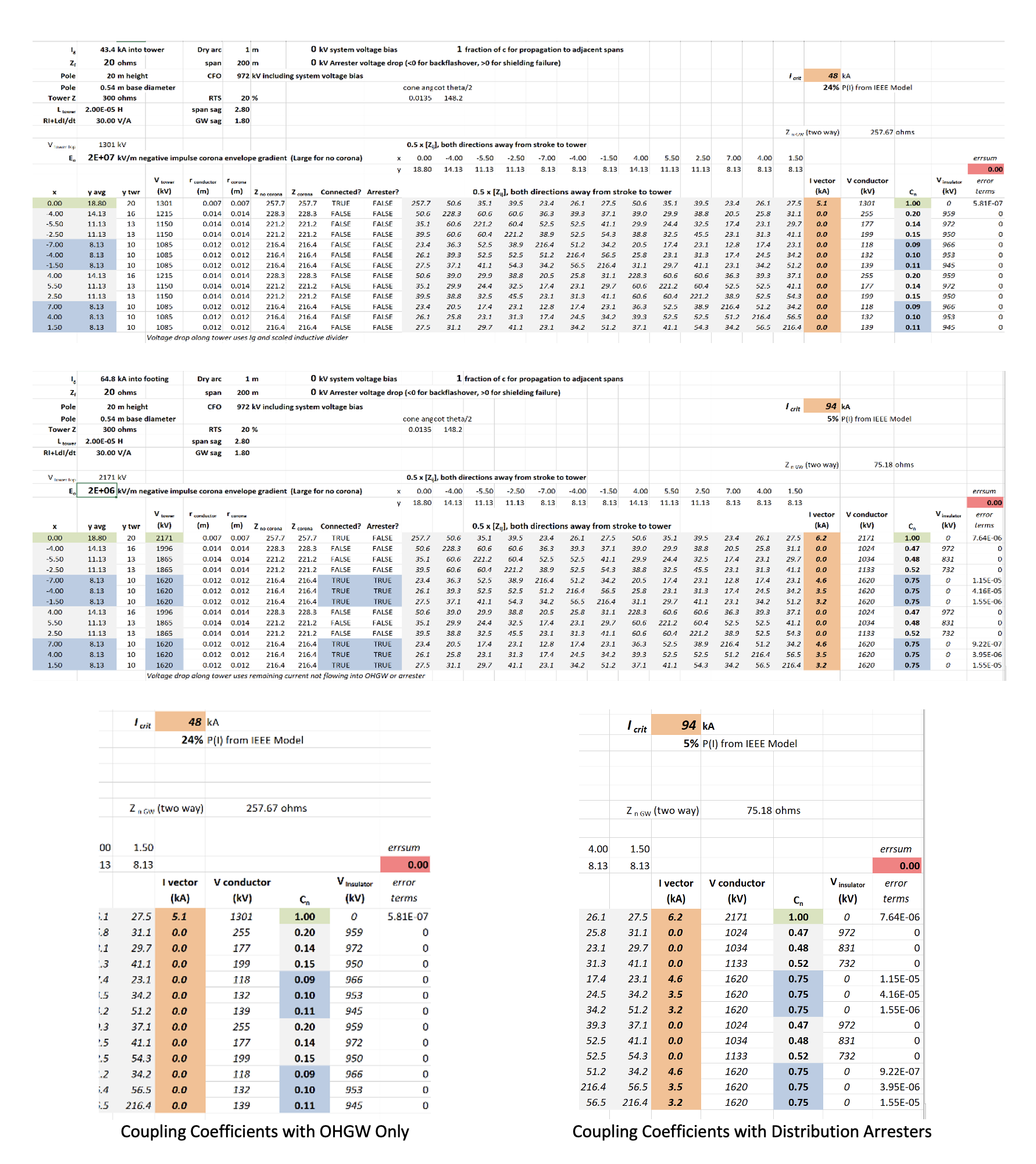
A quick estimate of the changes in coupling coefficient and increases in critical current can be made by altering the current vector in Fig. 7 to have unit currents in each protected phase. The spreadsheet elements in Fig. 4 to Fig. 7 were compacted into Fig. 8. The coupling coefficients and critical currents agree for single OHGW configuration. Then, the vector of currents is adjusted in Fig. 8 so that currents also flow into each of the six distribution system phase conductors.
Each surge impedance matrix value in Fig. 8 is exactly half of the values in Fig. 6. In the consolidation, the formulas implemented the fact that equal currents flow in two directions away from the tower into any OHGW or conductor that has been protected with an LSA. Also, voltages that appear on the bottom cross-arm in Fig. 1, highlighted in blue in Fig. 8 are lower than the voltage at tower top highlighted in green because the inductance from bottom cross-arm to the ground is lower.
Fig. 8 shows that the value of Icrit for the transmission circuits increases from 48 to 94 kA when ideal arresters are fitted to all six phases of the two distribution circuits. This would give a factor of five improvement in the lightning outage rate, based on the change in probability from 24% down to 5%. This compares favorably with some grounding improvement campaigns in terms of capital and maintenance costs as well as long-term effectiveness.
Further Improvement in Coupling: Impulse Corona
Under ordinary operating conditions, high voltage engineers understand that high local electric fields can cause partial discharges such as corona. The corona may be benign, for example an ultraviolet signature at the end of a cotter key on an insulator cap. In some conditions, such as heavy rain, the corona may be intense, with distinctive audible noise as well as a broadband electromagnetic radiation from the conductor-antenna gaps. The corona may be an indication of ongoing damage to insulators. Technologies of solar-blind ultraviolet cameras can sometimes distinguish a corona source. Generally, lines should be free of corona in clear, dry conditions and this makes UV cameras an important line inspection tool.
Under lightning surge conditions, corona switches from “enemy” to “friend”. The high voltages computed using the model in Fig. 2 cause envelopes of corona to form around towers and conductors. These have three main effects:
• Corona causes an increase in capacitance to ground, which reduces the parallel surge impedance Zn GW of any overhead groundwires and any arrester-protected phases
• Corona causes an increase in coupling coefficients from the driven (OHGW or arrester protected distribution phase) to undriven (unprotected transmission phase) conductors
• Corona (in the form of soil ionization) can reduce the footing impedance Zf for large currents
The fourth effect, of effectively slowing down the propagation speed to adjacent spans, is not helpful and is discussed separately.
One of the most interesting differences between IEEE and CIGRE practice is treatment of corona. The IEEE includes corona on the overhead wires with a simplified model, and pretty much ignores it when evaluating footing impedance, using the rationale that the currents required to make substantial soil ionization are too large to be relevant to the backflashover calculation. By contrast, CIGRE makes the corona effects on the OHGW difficult to model in electromagnetic transient programs, but their TB 63 does include a simple model for soil ionization.
We start with a gradient at the edge of the corona envelope, Eo and this was set to Eo =1500 kV/m for negative polarity. The corona radius Rc (m) is then given by:
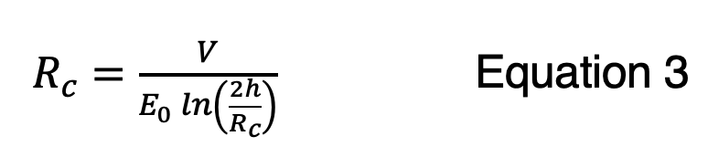 Where h is the average height above ground (m) and V is the applied voltage. If Rc is less than the physical radius of the conductor, there is no corona and no change to the surge impedance matrix. Equation 3 is ‘recursive’, that is the value of Rc appears on both sides of the equal sign. However, it has an interesting feature that makes it easy to use in the Excel model. The value of Rc converges rapidly. Any initial starting point – for example RC = 1 m – can be used. Then, an adjacent cell computes a new value of Rc. After five such calculations, each time using the fresh value of Rc, the final value is obtained. This is essentially a closed-form solution, and the function MAX(Rc, rconductor) will finalize the model so that low-current events do not cause corona but large-current events do.
The corona envelope modifies only the capacitance term in the surge impedance expression. This means that the self-surge impedance under corona will be:
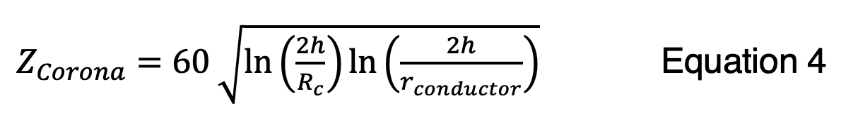
Corona-modified coupling was disabled in the calculations of Figure 8 by setting Eo to a large value, 2E+06. This ensured that Rc was smaller than rconductor , and the larger of the two values was used in computing ZCorona. When the recommended value of Eo = 1500 kV/m for negative polarity is substituted, Fig. 9 shows that the critical current increases from 94 kA to 120 kA mainly because the coupling coefficients for the transmission circuit increase from 0.47 £ Cn £ 0.52 to 0.55 £ Cn £ 0.60. There is also a modest reduction in Zn GW from 75 W to 65 W.
using Corona Envelope Gradient E0 = 1500 kV/m
Influence of Transmission Circuit Instantaneous Line Voltage
Lightning tends to have negative polarity in most regions through most of the year. Fig. 10 shows that the instantaneous ac power system voltage may be positive or negative, depending on phase and phase angle. At least one of the phases will have positive voltage, which will add to the stress on the insulator under lightning conditions. For reference, typical lightning duration of 100 ms corresponds to a bit more than 2° at 60 Hz in Fig. 10.
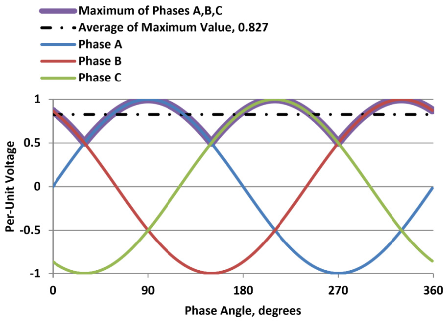
The maximum of phases A, B and C, averaged over the entire 360° period, gives a value of 0.827 per-unit (pu), where 1 pu is the maximum of the line-to-ground voltage as shown. Rather than carrying out calculations for each value of phase angle, the influence of system voltage can be treated simply by subtracting 0.827 pu from the critical flashover voltage.
The CFO in Fig. 9 was 972 kV. When the voltage bias from a 115 kV transmission system is included in Fig. 11, the CFO is effectively reduced by 0.827 ´ Ö2 ´ (115 kV)/ Ö3 to 895 kV. With greater stress across the insulators, we expect that the critical current will decrease and it does – dropping from Icrit=120 kA in Fig. 11 to Icrit=109 kA in Fig. 11.
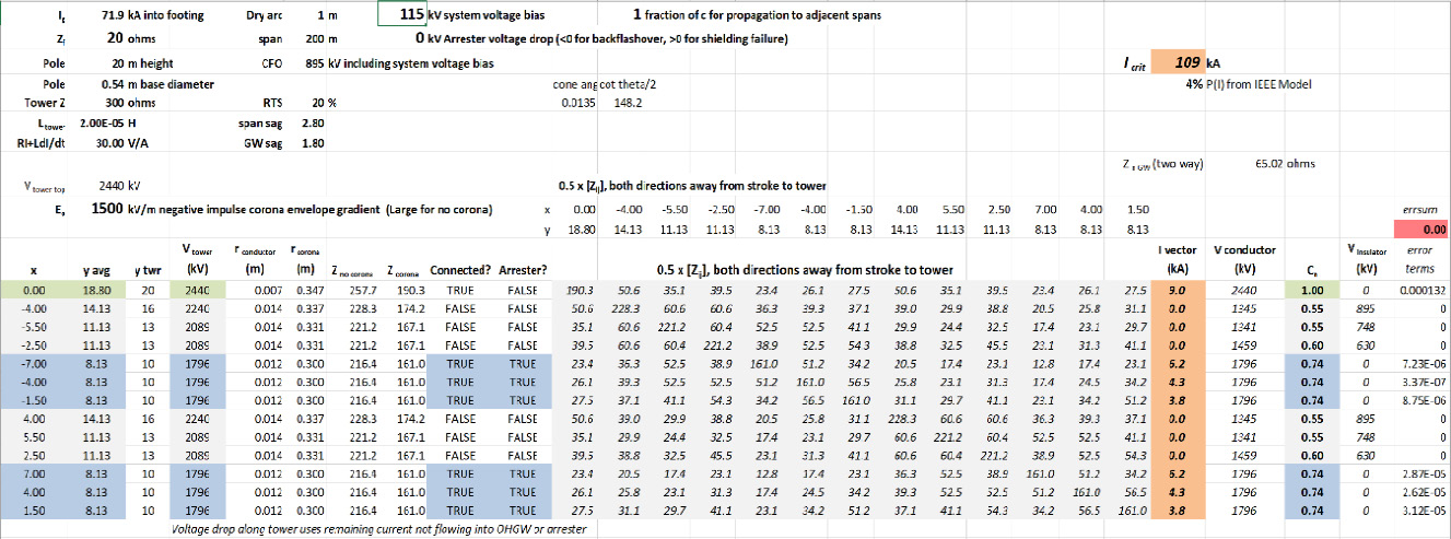
The probability of exceeding Icrit = 109 kA with ac system voltage bias remains low, 4% in Fig. 11 compared to 3% without line voltage in Fig. 10. This good performance relies on the low value of Zf = 20 W along with the benefits of six arresters on the two distribution circuits, giving coupling coefficients of 0.55 to 0.6 on the transmission phases that are unchanged from previous calculations using the same Eo = 1500 kV/m for corona envelope gradient.

Influence of Corona-Modified Propagation Velocity
The value of insulator voltage VPk used in Fig. 2 to compute Icrit is based on the insulator dry arc distance and the time of breakdown. For porcelain insulators, the strength is usually evaluated using a flashover time of 2 ms, at a gradient of 822 kV per meter, rather than the critical lightning impulse flashover gradient of 520 to 560 kV per meter. The time used in the volt-time curve adjustment is considered to be the time that cancelling reflections return from the adjacent two structures. This two-way travel time is a function of span length and can be as short as 0.7 ms for 100-m spans, or up to 2.7 ms for 400-m spans.
Tests that applied lightning impulses to conductors established that there is a continuous increase in the observed rise time for the portion of the voltage above the corona threshold. This effect that can be treated by assuming the propagation speed is somewhat less than the speed of light. The delay holds up stress on the insulators of the stricken tower for longer duration. Speed of propagation to 90% of the speed of light (0.9 c) was adjusted in Fig. 12.
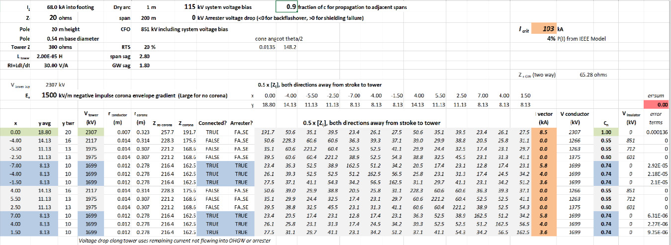
using corona envelope gradient E¬o = 1500 kV/m, 115 kV AC line voltage bias and corona-retarded propagation of 0.9c along spans.
The CFO including system voltage bias in Fig. 12, comparable to Fig. 11, drops from 895 kV to 951 kV. The critical current drops from Icrit = 109 kA in Fig. 11 to Icrit = 103 kA in Fig. 12 but the effect on the probability of exceeding Icrit is minimal, staying at 4% for both cases.
Influence of Surge Arrester Voltage Drop
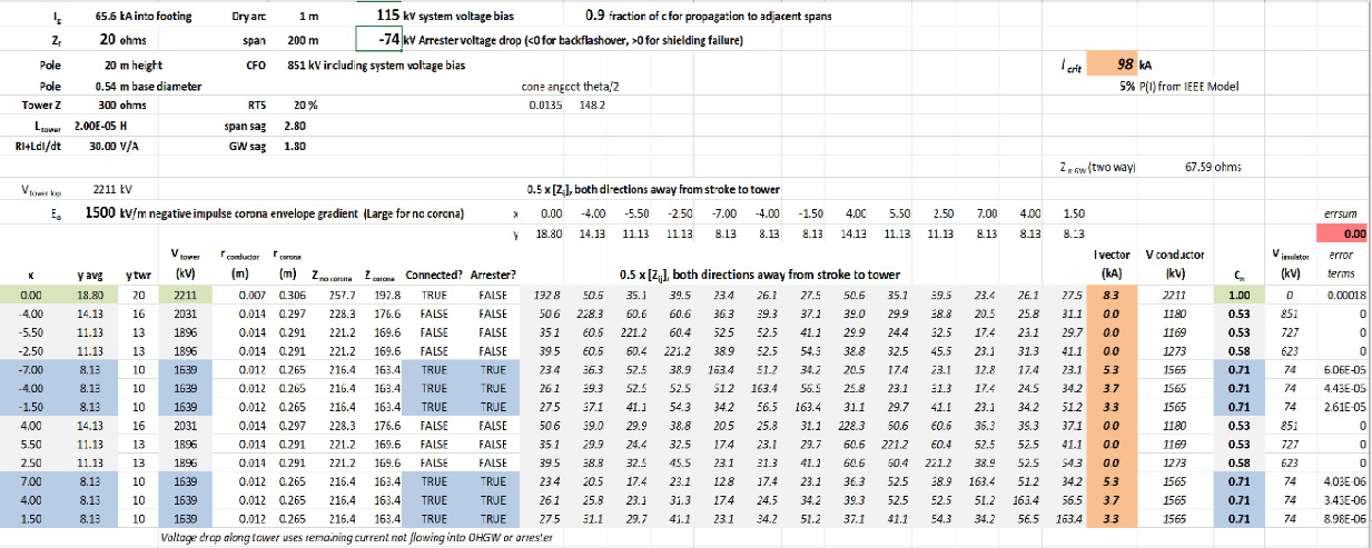
The solution vectors of currents in Figs. 9, 11 & 12 suggest that a current in the range of 4 to 7 kA will flow into each distribution circuit LSA. There will be a voltage drop associated with this current flow that should be subtracted from the voltages that appear on each phase. A typical 33 kV MCOV LSA has a voltage of about 74 kV with 5 kA current, rising to 87 kV at 10 kA and 101 kV at 20 kA. The voltage drop was entered in the highlighted cell of Fig. 13.
For this situation, the voltage drop across the distribution system line arresters reduces the voltages that will appear on these phases from 1699 kV in Fig. 12 to 1565 kV in Fig. 13. There are corresponding reductions in the currents that flow into each protection distribution phase and in the values of coupling coefficients Cn for the transmission circuits. The overall effect is a reduced value of Icrit = 98 kA and 5% probability of exceeding this.
A reference back to Fig. 8 confirms that the original estimate of Icrit, disregarding the benefits of corona-modified coupling, the line voltage bias, the slow propagation velocity with corona and the effect of arrester voltage drop, gave about the same value ICrit = 94 kA in this case. This is something worth checking in any simplified or detailed evaluation of the backflashover process.
Effect of Footing Impedance Zf on Results
Above, it has been stressed that the variation of Zf from tower to tower is random and governed by a log-normal distribution. Low-current footing impedance varied from 19 to 421 W in a typical simulation of nine towers in Fig. 3. To close out the section on modeling of the backflashover process, the simplified model (no corona effects, no system voltage bias, no arrester voltage drop) will be compared with the evaluation, following Fig. 13, using all these factors.
With and Without Arresters on Underbuilt Distribution Circuits
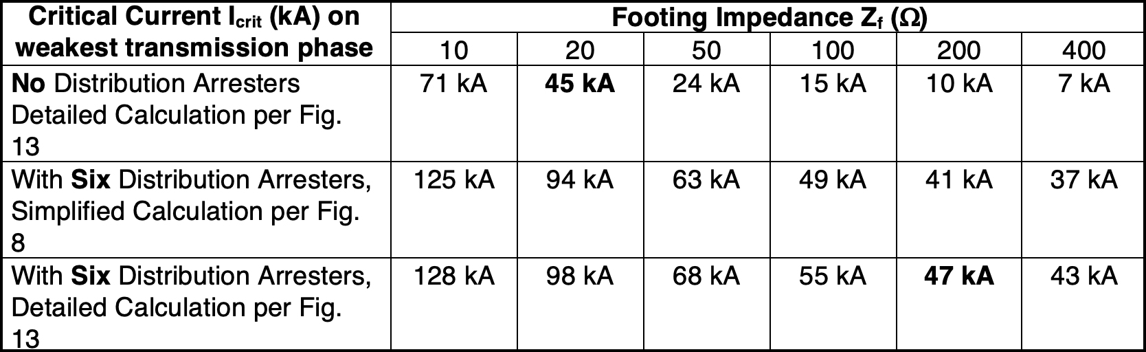
A line constructed with arresters and 200 Ω footing impedance would have the same performance as a line with 20 Ω footing impedance and no arresters on the underbuilt distribution circuit, based on similar values of Icrit in Table 1
The industry is in the process of deciding whether soil ionization effects or frequency dependence of soil resistivity offers the better explanation for the performance of transmission lines with high footing impedance. Both effects reduce Zf from a measured low current, low frequency value. For a simulation in Fig. 3 with r=250 Wm, the Korsuncev ionization model suggests that interface of the small monopole to the soil will start to ionize at a current well below our anticipated Icrit level, such that Zf for 30 kA may be less than half of the low-current values. In contrast to this modeling, which is very difficult to support with testing, the effects of frequency-dependent resistivity can and have been verified in many practical field studies as described in the work of CIGRE Working Group C4.33. A final issue is a composite of both effects: it is anticipated that the corona envelope of ionization in the soil will support a higher gradient of up to 1500 kV/m in dense, rocky soil compared to 400 kV/m in low resistivity soil.
Mechanical Aspects of Arresters on Underbuilt Distribution
The insulators in Fig. 1 restrain some horizontal movements of the conductors, making this by EPRI-USA definition a “compact” design. Rigid or semi-rigid insulators reduce the possibility of conductor-to-conductor contacts. They also simplify the installation of line surge arresters (LSA) in parallel, to limit lightning overvoltages and prevent flashovers.
For example, a 1990s non-gapped line arrester (NGLA) concept from Hydro-Québec in Fig. 14 shows a metal support plate bolted between a pedestal-post non-ceramic insulator and the conductor support. A suitably rated 39 kV MCOV arrester hangs off the end of this plate. At the bottom of the arrester, there is a flexible AWG 4 copper ground lead, also about 750 mm long, attached to an explosive disconnect module on the bottom of the arrester. The rigid mount above and short lead length below mitigate many issues with flexing, vibration and fatigue.
Since the late 1990s, when this sub-transmission-system arrester concept was explored, LSAs have been developed further and applied successfully on many transmission lines. The term “TLSA” has been reserved for transmission-level voltages, usually shielded lines with phase to phase voltage of at least 69 kV. The mechanical configuration suggested in Fig. 14 has been successfully:
• Rotated 90°, so that the arrester hangs below a horizontal post insulator;
• Inverted, so that a davit arm supports a TLSA from below; and
• Doubled, with support arms at each end of an insulator, two TLSA and a series air gap between them to form an externally gapped line arrester (EGLA).

Connecteur de MALT = ground lead; Isolateur composite = composite insulator (NCI); Parafoudre de ligne = Line Surge Arrester (LSA); Plaque de support = support plate
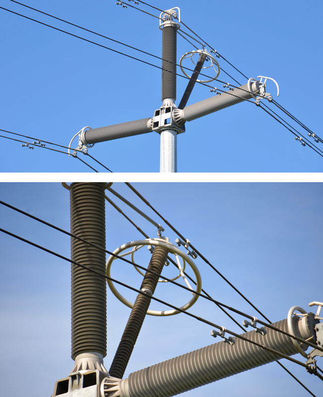
A close-up of the well-known application of 400 kV TLSA on a few spans in Norway shows a similar, semi-rigid metal strap that holds the upper end of the arrester body away from the head of the post insulator. The 400 kV TLSA support arm in Fig. 15 is located between the twin phase conductors, in an equipotential zone that can eliminate problems with corona around small-radius features. Connection bolts at the head of the arrester are further shielded by a pair of corona rings.
In addition to shielding of mechanical parts by corona rings, projects to apply TLSA should keep in mind the conductor tension. Many transmission line circuits are engineered with maximum tensions on the order of 20% of the rated tensile strength (RTS) of the conductor, where distribution system engineers are more familiar with lines strung at 5-10% RTS. Higher tensions may lead to possible problems with Aeolian vibration. The interaction of TLSA with vibration dampers has been discussed as an application problem by CIGRE. A prescient feature of the mounting arrangements in Figs. 14 and 15 is that the arrester mounting does not interfere with the vibration dampers. In Fig. 15, the twelve Aeolian vibration dampers are the pairs of weights, connected by a wire and mounted a short distance on each side of the conductor clamps.
Dealing with Cross-Circuit Contacts
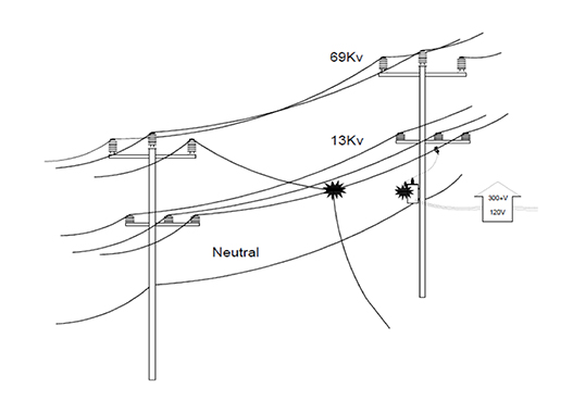
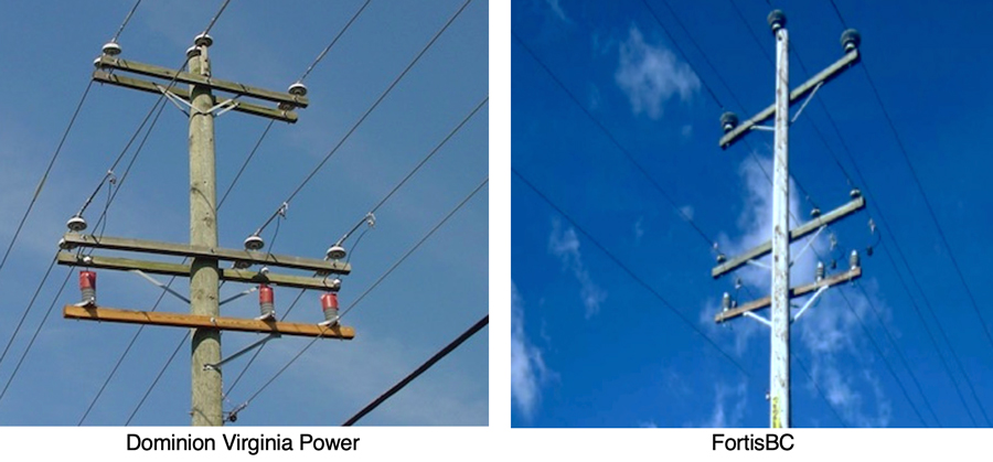
INMR has presented several articles describing a concept, originating at Dominion Virginia Power and also adopted at Fortis BC, that makes use of arresters on a distribution circuit to protect from cross-circuit faults. The schematic in Fig. 16 shows the problem of a broken conductor on an unshielded 69 kV line that contacts the 13 kV phase below. This will generate substantial and unexpected overvoltages that may have long duration if relays do not recognize the unusual condition quickly.
The proposed mitigation was to provide sacrificial surge arresters that would fail in a predictable way, called a ‘crowbar’ configuration to ensure a low-impedance line-to-ground fault. Fig. 17 shows the implementations of this concept, using station class distribution system arresters at periodic intervals.
Light-duty arresters could be considered for protecting the distribution circuits in Fig. 1, especially considering that the highest peak currents flowing in the arresters wound be around 5 kA. However, there is no guarantee that several light-duty arresters in parallel would share the exceptionally large charge duty from a transmission line contact equally. There are some options to consider for combining both protection schemes in a single retrofit:
• Using distribution arresters with two different voltage and energy ratings, especially fitting heavy-duty arresters with lower MCOV at selected poles with low soil resistivity and Zf, or
• Relying on a cascade of light-duty arrester failures to provide the desired long-duration low-impedance path to ground.

Conclusions
Placing surge arresters on all six phases of the two distribution circuits in Fig. 1 makes a significant increase in the coupling coefficients to the unprotected transmission circuits. It is computed that the critical current would double, leading to a factor of five improvement in transmission line outage rate, when a cooperation is made to allow such an underbuilt distribution line.
A line constructed with arresters on all six distribution phases and 200 footing impedance would have the same performance as a line with 20 footing impedance and no arresters on the underbuilt distribution circuit.
Corona-modified coupling makes a significant improvement in calculated backflashover performance. However, most of this gain is clawed back when other factors, such as instantaneous system voltage bias, slow return of reflections from corona effects and non-zero voltage drop across LSA, are included in the backflashover calculation.
Rigid or semi-rigid mounting of surge arresters on distribution circuits is simplified in many cases if post insulators are used.
Fitting arresters on every insulator of a distribution underbuild also provides some degree of protection against cross-circuit contact. A successful retrofit may require the selection of station-class arresters, placed at 1-10 km intervals, that absorb most of the energy in cross-system contact exposure and fail in the desired short-circuit (crowbar) manner.
References
[1] INMR, “Gallery of Transmission Structures – Wallpaper Oct 16,” Zimmar Holdings Ltd. / INMR, October 2016. [Online]. Available: https://www.inmr.com/gallery/. [Accessed 10 07 2019].
[2] W. A. Chisholm and S. de Almeida de Graaff, “Adapting the Statistics of Soil Properties into Existing and Future Lightning Protection Standards and Guides,” in 2015 International Symposium on Lightning Protection (XIII SIPDA), Balneario Camboriu, Brazil, 28 September – 2 October 2015.
[3] IEEE, IEEE Guide for Improving the Lightning Performance of Transmission Lines, Piscataway, NJ: IEEE Standard 1243-1997, Reaffirmed 2008, September 2008.
[4] EPRI, Transmission Line Reference Book, 345 kV and Above, Second Edition, Palo Alto, CA: EPRI, 1982.
[5] CIGRE WG 33.01, Guide to Procedures for Estimating the Lightning Performance of Transmission Lines, Paris: CIGRE Technical Brochure 63, 1991.
[6] A. R. Hileman, Insulation Coordination for Power Systems, New York: Marcel Dekker Inc., 1999.
[7] EPRI, EPRI AC Transmission Line Reference Book – 200 kV and Above, Third Edition (the Red Book), Palo Alto, CA: EPRI 1011974, December 2005.
[8] EPRI, Transmission Line Reference Book: 115-345 kV Compact Line Design, Palo Alto, CA: EPRI 1016823, 2008.
[9] EPRI, “Guide for Transmission Line Grounding: A Roadmap for Design, Testing and Remediation,” EPRI, Palo Alto, CA, 2004. 1002021.
[10] CIGRE WG C4.407, Lightning Parameters for Engineering Applications, Paris: CIGRE Technical Brochure 549, August 2013.
[11] J. Takami and S. Okabe, “Observational Results of Lightning Current on Transmission Towers,” IEEE Transactions on Power Delivery, vol. 22, no. 1, pp. 547-556, January 2007.
[12] W. Chisholm and W. Janischewskyj, “Lightning Surge Response of Ground Electrodes,” IEEE Transactions on Power Delivery, vol. 4, no. 2, pp. 1329-1337, April 1989.
[13] CEATI Technologies, “Guidelines for the Installation of Surge Arresters on Sub-Transmission and Transmission Lines using Different Structure Designs at Voltages from 69 kV to 345 kV,” CEATI Report T033700-3312A, Montreal, March 2005.
[14] D. Havard, P. Dulhunty, G. Diana, K. Halsan, H.-J. Krispin, J.-P. Paradis, D. Sunkle, B. Wareing, G. Chapman, W. Chisholm, U. Cosmai, T. Furtado, A. Goel, J. Lundquist, R. L. Markiewicz, M. Mito, C. Rozé and e. al., “Interaction of vibration dampers with surge arresters,” CIGRE Science and Engineering, vol. 6, no. 4, pp. 32-45, October 2016.
[15] D. J. Ward, “Overvoltage Protectors – A Novel Concept for Dealing with Overbuilt Distribution Circuits,” IEEE Transactions on Power Delivery, vol. 25, no. 3, pp. 1971-1977, July 2010.
[16] INMR, “Application of Station Class Arresters on Underbuilt Distribution Lines,” 19 06 2018. [Online]. Available: https://www.inmr.com/application-station-class-arresters-underbuilt-distribution-lines-3. [Accessed 05 07 2019].