Coming at the 2025 INMR WORLD CONGRESS
The ongoing energy transition requires major investments in connections and resilience. Such transitions and trends add to the requirements of the grid and as such also impose a threat to reliability and performance of the grid.
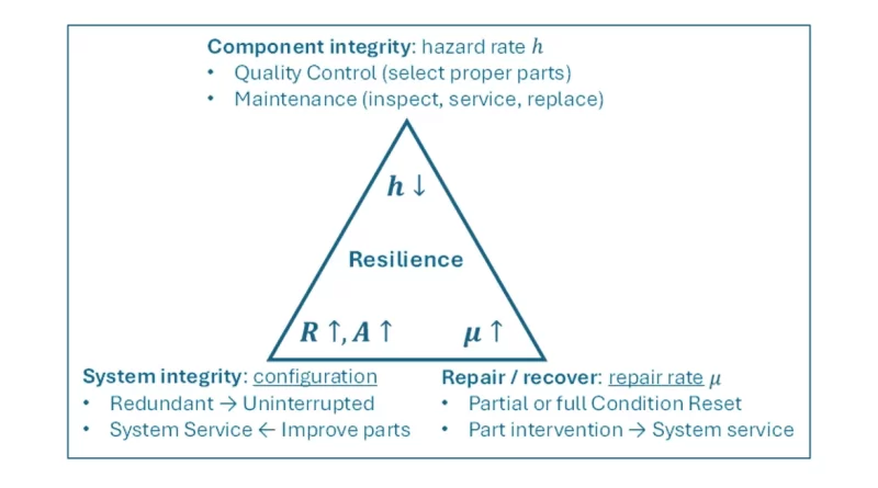
Technological approaches to support system resilience can be divided into three basic categories: component integrity, system integrity and recovery. These categories influence resilience and can at least partially compensate for one another. This is represented by the so-called ‘resilience triangle approach’.
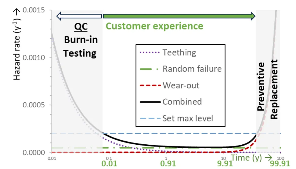
Reliability is often expressed in terms of remaining useful life (RUL) or probability of failure. Utilities increasingly use the method of asset health index (HI) and other indices to support decision-making in replacement and refurbishment. CIGRE, for example, has produced brochures where health index balances between RUL, probabilities and hazard rates. Since hazard rate is an especially useful function basic to any treatment of reliability and availability, below is a brief review of hazard rate, the hazard rate bathtub curve and repair rate.
Hazard Rate as Measure of Quality
A statistical failure distribution describes how failure of a group of items is distributed over time, t. The fraction of failed items is shown by the cumulative failure function F(t) and the still functional fraction by the reliability (also: survival) function R(t) = 1 – F(t). At the start of operation t=0, usually, a group is taken to be fully functional, i.e., F(0)=0% and R(0)=100%. The rate at which the fraction of failed items grows is the failure density function f(t), the time derivative of F:
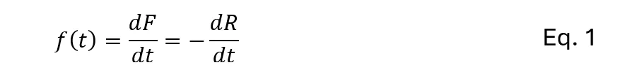
When the surviving fraction drops well below 100%, main interest is usually not on growth rate with respect to total group of items but rather on the rate with respect to only the as-yet-surviving items. This is the hazard rate h(t).
![]()
Hazard rate is the probability that as-yet-working items will fail over a defined coming period. A typical example of a hazard rate statement is: ‘it is estimated that 0.1% of presently working items X will fail in the coming one year’.
There may be criteria for acceptable hazard rate levels, e.g. how many failures are acceptable to a series of products or circuits in the next year or hazard rate levels at which replacement or maintenance is needed. This hazard rate is equal to the number of failures in each period divided by the number of still working items.
However, it is not only failure that can be described by a hazard rate. Also, repair can be viewed as a component or system being in a state of not yet being repaired and a repair rate to transition to the other state (i.e. being repaired). Rates are often taken as a constant (resembling the random failure phase). More advanced, time-varying rates can also be employed.
Plan to attend the upcoming 2025 INMR WORLD CONGRESS in Panama, where one of the speakers will be reliability and asset management expert, Prof. Robert Ross of the IWO Institute for Science & Development in the Netherlands. Dr. Ross will discuss challenges to asset management in the light of the energy transition. Based on latest Research, Development and Innovation needs, as described by the network of European TSOs, he will review enhancement of reliability and explain the resilience triangle. This is a concept for comparing the contributions of component integrity by quality, system integrity by configuration and recovery rate through proper strategies.